Jupyter Notebook
Kleis provides Jupyter kernel support, allowing you to write and execute Kleis code in Jupyter notebooks. This is ideal for:
JupyterLab launcher with Kleis and Kleis Numeric kernels
- Interactive exploration of mathematical concepts
- Teaching mathematical foundations
- Documenting proofs and derivations
- Numerical computation with LAPACK operations
- Publication-quality plotting with Lilaq/Typst integration
Quick Start
cd kleis-notebook
./start-jupyter.sh
This will:
- Create a Python virtual environment (if needed)
- Install JupyterLab and the Kleis kernel
- Launch JupyterLab in your browser
Installation
Prerequisites
- Python 3.8+ with pip
- Kleis binary compiled with numerical features:
cd /path/to/kleis
export Z3_SYS_Z3_HEADER=/opt/homebrew/opt/z3/include/z3.h  # macOS Apple Silicon
cargo install --path . --features numerical
Note: The
--features numericalflag enables LAPACK operations for eigenvalues, SVD, matrix inversion, and more.
Install the Kernel
cd kleis-notebook

# Option 1: Use the launcher script (recommended)
./start-jupyter.sh install

# Option 2: Manual installation
python3 -m venv venv
source venv/bin/activate
pip install -e .
pip install jupyterlab
python -m kleis_kernel.install
python -m kleis_kernel.install_numeric
Using Kleis in Jupyter
Creating a Notebook
- Start JupyterLab:
./start-jupyter.sh - Click New Notebook
- Select Kleis or Kleis Numeric kernel
Example: Defining a Group
structure Group(G) {
    operation (*) : G × G → G
    element e : G

    axiom left_identity: ∀(a : G). e * a = a
    axiom right_identity: ∀(a : G). a * e = a
    axiom associativity: ∀(a b c : G). (a * b) * c = a * (b * c)
}
Example: Testing Properties
example "group identity" {
    assert(e * e = e)
}
Output:
✅ group identity passed
Example: Numerical Computation
eigenvalues([[1.0, 2.0], [3.0, 4.0]])
Output:
[-0.3722813232690143, 5.372281323269014]
REPL Commands
Use REPL commands directly in notebook cells:
| Command | Description | Example |
|---|---|---|
:type <expr> | Show inferred type | :type 1 + 2 |
:eval <expr> | Evaluate concretely | :eval det([[1,2],[3,4]]) |
:verify <expr> | Verify with Z3 | :verify ∀(x : ℝ). x + 0 = x |
:ast <expr> | Show parsed AST | :ast sin(x) |
:env | Show session context | :env |
:load <file> | Load .kleis file | :load stdlib/prelude.kleis |
Jupyter Magic Commands
| Command | Description |
|---|---|
%reset | Clear session context (forget all definitions) |
%context | Show accumulated definitions |
%version | Show Kleis and kernel versions |
Numerical Operations
When Kleis is compiled with --features numerical, these LAPACK-powered operations are available:
Eigenvalue Decomposition
// Compute eigenvalues
eigenvalues([[4.0, 2.0], [1.0, 3.0]])
// → [5.0, 2.0]

// Full decomposition (eigenvalues + eigenvectors)
eig([[4.0, 2.0], [1.0, 3.0]])
// → [[5.0, 2.0], [[0.894, 0.707], [-0.447, 0.707]]]
Matrix Factorizations
// Singular Value Decomposition
svd([[1.0, 2.0], [3.0, 4.0], [5.0, 6.0]])
// → (U, S, Vt)

// QR Decomposition
qr([[1.0, 2.0], [3.0, 4.0]])
// → (Q, R)

// Cholesky Decomposition (symmetric positive definite)
cholesky([[4.0, 2.0], [2.0, 5.0]])
// → Lower triangular L where A = L * L^T

// Schur Decomposition
schur([[1.0, 2.0], [3.0, 4.0]])
// → (U, T, eigenvalues)
Linear Algebra
// Matrix inverse
inv([[1.0, 2.0], [3.0, 4.0]])
// → Matrix(2, 2, [-2, 1, 1.5, -0.5])

// Determinant
det([[1.0, 2.0], [3.0, 4.0]])
// → -2

// Solve linear system Ax = b
solve([[3.0, 1.0], [1.0, 2.0]], [9.0, 8.0])
// → [2.0, 3.0]

// Matrix rank
rank([[1.0, 2.0, 3.0], [4.0, 5.0, 6.0], [7.0, 8.0, 9.0]])
// → 2

// Condition number
cond([[1.0, 2.0], [3.0, 4.0]])
// → 14.933...

// Matrix norms
norm([[1.0, 2.0], [3.0, 4.0]])
// → Frobenius norm
Matrix Exponential
// e^A (useful for differential equations)
expm([[0.0, 1.0], [-1.0, 0.0]])
// → rotation matrix
Built-in Functions Reference
Important: These functions perform concrete numeric computation. They cannot be used in symbolic contexts such as
structuredefinitions,axiomdeclarations, or abstract proofs. They are designed for interactive exploration, plotting, and numerical analysis.
Math Functions
| Function | Description | Example |
|---|---|---|
sin(x) | Sine (radians) | sin(3.14159) → 0.0 |
cos(x) | Cosine (radians) | cos(0) → 1.0 |
sqrt(x) | Square root | sqrt(2) → 1.414... |
pi() | π constant | pi() → 3.14159... |
radians(deg) | Degrees to radians | radians(180) → 3.14159... |
mod(a, b) | Modulo operation | mod(7, 3) → 1 |
Sequence Generation
| Function | Description | Example |
|---|---|---|
range(n) | Integers 0 to n-1 | range(5) → [0, 1, 2, 3, 4] |
range(start, end) | Integers start to end-1 | range(2, 5) → [2, 3, 4] |
linspace(start, end) | 50 evenly spaced values | linspace(0, 1) → [0, 0.02, ...] |
linspace(start, end, n) | n evenly spaced values | linspace(0, 1, 5) → [0, 0.25, 0.5, 0.75, 1] |
Random Number Generation
These use a deterministic pseudo-random number generator (LCG) for reproducibility.
| Function | Description | Example |
|---|---|---|
random(n) | n uniform random values in [0,1] | random(5) → [0.25, 0.08, ...] |
random(n, seed) | With explicit seed | random(5, 42) → reproducible |
random_normal(n) | n values from N(0,1) | random_normal(5) |
random_normal(n, seed) | With explicit seed | random_normal(5, 33) |
random_normal(n, seed, scale) | N(0, scale) | random_normal(50, 33, 0.1) |
Vector Operations
| Function | Description | Example |
|---|---|---|
vec_add(a, b) | Element-wise addition | vec_add([1,2,3], [4,5,6]) → [5, 7, 9] |
List Manipulation
| Function | Description | Example |
|---|---|---|
list_map(f, xs) | Apply f to each element | list_map(λ x . x*2, [1,2,3]) → [2, 4, 6] |
list_filter(p, xs) | Keep elements where p(x) is true | list_filter(λ x . x > 1, [1,2,3]) → [2, 3] |
list_fold(f, init, xs) | Left fold/reduce | list_fold(λ a b . a + b, 0, [1,2,3]) → 6 |
list_zip(xs, ys) | Pair corresponding elements | list_zip([1,2], ["a","b"]) → [Pair(1,"a"), ...] |
list_nth(xs, i) | Element at index i (0-based) | list_nth([10,20,30], 1) → 20 |
list_length(xs) | Number of elements | list_length([1,2,3]) → 3 |
list_concat(xs, ys) | Concatenate two lists | list_concat([1,2], [3,4]) → [1, 2, 3, 4] |
list_flatten(xss) | Flatten nested lists | list_flatten([[1,2], [3,4]]) → [1, 2, 3, 4] |
list_slice(xs, start, end) | Sublist [start, end) | list_slice([0,1,2,3,4], 1, 3) → [1, 2] |
list_rotate(xs, n) | Rotate left by n | list_rotate([1,2,3,4], 1) → [2, 3, 4, 1] |
Pair Operations
| Function | Description | Example |
|---|---|---|
Pair(a, b) | Create a pair/tuple | Pair(1, "x") |
fst(p) | First element of pair | fst(Pair(1, 2)) → 1 |
snd(p) | Second element of pair | snd(Pair(1, 2)) → 2 |
Why Numeric-Only?
These functions are implemented in Rust for performance and produce concrete values:
// ✅ Works: Concrete computation
let xs = linspace(0, 6.28, 10)
let ys = list_map(λ x . sin(x), xs)
diagram(plot(xs, ys))

// ❌ Does NOT work: Cannot use in axioms
structure MyStructure(T) {
    axiom bad: sin(x) = cos(x - pi()/2)  // ERROR: sin/cos/pi are numeric
}
For symbolic mathematics, define your own abstract operations:
// ✅ Correct: Define sin symbolically
structure Trigonometry(T) {
    operation sin : T → T
    operation cos : T → T
    constant π : T

    axiom shift: ∀(x : T). sin(x) = cos(x - π/2)
}
Matrix Syntax
Matrices can be specified using nested list syntax:
// 2×2 matrix (row-major order)
[[1, 2], [3, 4]]

// 3×3 identity matrix concept
[[1, 0, 0], [0, 1, 0], [0, 0, 1]]

// Column vector as 3×1 matrix
[[1], [2], [3]]

// Row vector as 1×3 matrix
[[1, 2, 3]]
Session Persistence
Definitions persist across cells within a session:
Cell 1:
define square(x) = x * x
Cell 2:
example "use square" {
    assert(square(3) = 9)
}
Output:
✅ use square passed
Use %reset to clear all definitions and start fresh.
Tips for Effective Notebooks
- Start with imports and definitions at the top
- Use example blocks for testable assertions
- Use
:evalfor quick numerical calculations - Use
:verifyfor Z3-backed proofs - Document with markdown cells between code
- Save frequently - Kleis notebooks are standard
.ipynbfiles
Troubleshooting
“kleis binary not found”
Install Kleis with:
cd /path/to/kleis
export Z3_SYS_Z3_HEADER=/opt/homebrew/opt/z3/include/z3.h
cargo install --path . --features numerical
Numerical operations return symbolic expressions
Make sure Kleis was compiled with --features numerical:
cargo install --path . --features numerical
Kernel dies unexpectedly
Check the terminal for error messages. Common causes:
- Z3 timeout on complex verification
- Memory issues with large matrices
Imports fail (stdlib not found)
When running Jupyter from a directory other than the Kleis project root, stdlib imports may fail:
Error: Cannot find file: stdlib/prelude.kleis
Solution: Set the KLEIS_ROOT environment variable to point to your Kleis installation:
export KLEIS_ROOT=/path/to/kleis
jupyter lab
Or add it to your shell profile (~/.bashrc, ~/.zshrc):
export KLEIS_ROOT="$HOME/git/cee/kleis"
The Kleis kernel automatically searches for stdlib in:
$KLEIS_ROOT/stdlib/(if KLEIS_ROOT is set)- Current working directory
- Parent directories (up to 10 levels)
Unicode input
Use standard Kleis Unicode shortcuts:
\forall→∀\exists→∃\in→∈\R→ℝ\N→ℕ\Z→ℤ
Example Notebook
Here’s a complete example exploring matrix properties:
Cell 1: Setup
// Define a 2×2 matrix
let A = [[1.0, 2.0], [3.0, 4.0]]
Cell 2: Basic properties
det(A)        // → -2
trace(A)      // → 5 (not yet implemented, use 1+4)
Cell 3: Eigenvalues
eigenvalues(A)
// → [-0.372..., 5.372...]
Cell 4: Verify Cayley-Hamilton
// A matrix satisfies its characteristic polynomial
// For 2×2: A² - trace(A)*A + det(A)*I = 0
// This is verified numerically by the eigenvalue product
Cell 5: Matrix inverse
let Ainv = inv(A)
// Verify: A * Ainv should be identity
// (Matrix multiplication coming soon!)
Plotting
Kleis integrates with Lilaq (Typst’s plotting library) to generate publication-quality plots directly in Jupyter notebooks. The API mirrors Lilaq’s compositional design, making it easy to create complex visualizations.
Requirements
- Typst CLI must be installed:
brew install typst(macOS) or see typst.app - Lilaq 0.5.0+ is automatically imported
Compositional API
Kleis uses a compositional plotting API where:
- Individual functions (
plot,scatter,bar, etc.) create PlotElement objects - The
diagram()function combines elements and renders to SVG - Named arguments (
key = value) configure options
diagram(
    plot(xs, ys, color = "blue"),
    scatter(xs, ys, mark = "s"),
    bar(xs, heights, label = "Data"),
    title = "My Chart",
    xlabel = "X-axis",
    theme = "moon"
)
Plot Functions
| Function | Description | Example |
|---|---|---|
plot(x, y, ...) | Line plot | plot([0,1,2], [0,1,4], color = "blue") |
scatter(x, y, ...) | Scatter with colormaps | scatter(x, y, colors = vals, map = "turbo") |
bar(x, heights, ...) | Vertical bars | bar([1,2,3], [10,25,15], label = "Data") |
hbar(y, widths, ...) | Horizontal bars | hbar([1,2,3], [10,25,15]) |
stem(x, y) | Stem plot | stem([0,1,2], [0,1,1]) |
fill_between(x, y, ...) | Area under curve | fill_between(x, y1, y2 = y2) |
stacked_area(x, y1, y2, ...) | Stacked areas | stacked_area(x, y1, y2, y3) |
boxplot(d1, d2, ...) | Box and whisker | boxplot([1,2,3], [4,5,6]) |
heatmap(matrix) | 2D color grid | heatmap([[1,2],[3,4]]) |
contour(matrix) | Contour lines | contour([[1,2],[3,4]]) |
path(points, ...) | Arbitrary polygon | path(pts, fill = "blue", closed = true) |
place(x, y, text, ...) | Text annotation | place(1, 5, "Peak", align = "top") |
yaxis(elements, ...) | Secondary y-axis | yaxis(bar(...), position = "right") |
xaxis(...) | Secondary x-axis | xaxis(position = "top", functions = ...) |
Data Generation Functions
| Function | Description | Example |
|---|---|---|
linspace(start, end, n) | Evenly spaced values | linspace(0, 6.28, 50) |
range(n) | Integers 0 to n-1 | range(10) |
random(n, seed) | Uniform random [0,1] | random(50, 42) |
random_normal(n, seed, scale) | Normal distribution | random_normal(50, 33, 0.1) |
vec_add(a, b) | Element-wise addition | vec_add(xs, noise) |
Example: Grouped Bar Chart with Error Bars
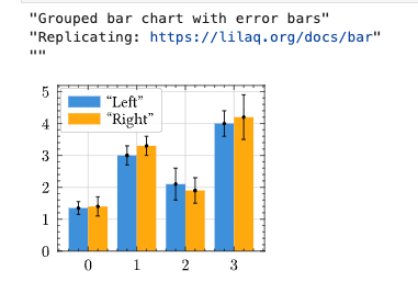
let xs = [0, 1, 2, 3]
let ys1 = [1.35, 3, 2.1, 4]
let ys2 = [1.4, 3.3, 1.9, 4.2]
let yerr1 = [0.2, 0.3, 0.5, 0.4]
let yerr2 = [0.3, 0.3, 0.4, 0.7]

let xs_left = list_map(λ x . x - 0.2, xs)
let xs_right = list_map(λ x . x + 0.2, xs)

diagram(
    bar(xs, ys1, offset = -0.2, width = 0.4, label = "Left"),
    bar(xs, ys2, offset = 0.2, width = 0.4, label = "Right"),
    plot(xs_left, ys1, yerr = yerr1, color = "black", stroke = "none"),
    plot(xs_right, ys2, yerr = yerr2, color = "black", stroke = "none"),
    width = 5,
    legend_position = "left + top"
)
Example: Bar Chart with Dynamic Annotations
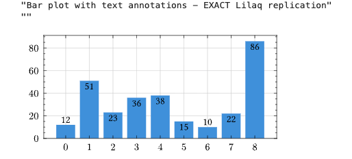
let xs = [0, 1, 2, 3, 4, 5, 6, 7, 8]
let ys = [12, 51, 23, 36, 38, 15, 10, 22, 86]

// Dynamic annotations using list_map and conditionals
let annotations = list_map(λ p .
    let x = fst(p) in
    let y = snd(p) in
    let align = if y > 12 then "top" else "bottom" in
    place(x, y, y, align = align, padding = "0.2em")
, list_zip(xs, ys))

diagram(
    bar(xs, ys),
    annotations,
    width = 9,
    xaxis_subticks = "none"
)
Example: Climograph with Twin Axes
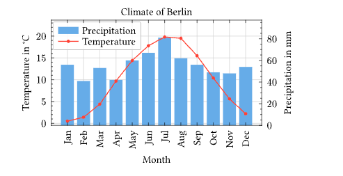
let months = ["Jan", "Feb", "Mar", "Apr", "May", "Jun",
              "Jul", "Aug", "Sep", "Oct", "Nov", "Dec"]
let precipitation = [56, 41, 53, 42, 60, 67, 81, 62, 56, 49, 48, 54]
let temperature = [0.5, 1.4, 4.4, 9.7, 14.4, 17.8, 19.8, 19.5, 15.5, 10.4, 5.6, 2.2]
let xs = range(12)

diagram(
    yaxis(
        bar(xs, precipitation, fill = "blue.lighten(40%)", label = "Precipitation"),
        position = "right",
        axis_label = "Precipitation in mm"
    ),
    plot(xs, temperature, label = "Temperature", color = "red", stroke = "1pt", mark_size = 6),
    width = 8,
    title = "Climate of Berlin",
    ylabel = "Temperature in °C",
    xlabel = "Month",
    xaxis_ticks = months,
    xaxis_tick_rotate = -90,
    xaxis_subticks = "none"
)
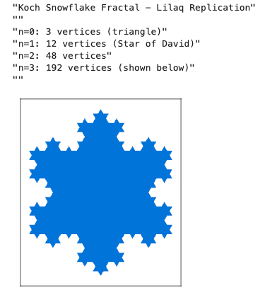
Example: Koch Snowflake Fractal
// Complex number operations
define complex_add(c1, c2) = Pair(fst(c1) + fst(c2), snd(c1) + snd(c2))
define complex_sub(c1, c2) = Pair(fst(c1) - fst(c2), snd(c1) - snd(c2))
define complex_mul(c1, c2) = Pair(
    (fst(c1)*fst(c2)) - (snd(c1)*snd(c2)),
    (fst(c1)*snd(c2)) + (snd(c1)*fst(c2))
)

define triangle_vertex(angle) = Pair(cos(radians(angle)), sin(radians(angle)))
define base_triangle() = [triangle_vertex(90), triangle_vertex(210), triangle_vertex(330)]

define koch_edge(p1, p2) =
    let d = complex_sub(p2, p1) in
    [p1, complex_add(p1, complex_mul(d, Pair(1/3, 0))),
     complex_add(p1, complex_mul(d, Pair(0.5, 0 - sqrt(3)/6))),
     complex_add(p1, complex_mul(d, Pair(2/3, 0)))]

define koch_iter(pts) =
    let n = list_length(pts) in
    list_flatten(list_map(λ i .
        koch_edge(list_nth(pts, i), list_nth(pts, mod(i + 1, n)))
    , range(n)))

let n0 = base_triangle()
let n3 = koch_iter(koch_iter(koch_iter(n0)))  // 192 vertices

diagram(
    path(n3, fill = "blue", closed = true),
    width = 6, height = 7,
    xaxis_ticks_none = true,
    yaxis_ticks_none = true
)
Example: Scatter Plot with Colormap
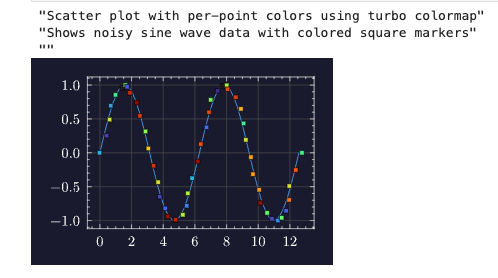
let xs = linspace(0, 12.566370614, 50)  // 0 to 4π
let ys = list_map(lambda x . sin(x), xs)
let noise = random_normal(50, 33, 0.1)
let xs_noisy = vec_add(xs, noise)
let colors = random(50, 42)

diagram(
    plot(xs, ys, mark = "none"),
    scatter(xs_noisy, ys,
        mark = "s",
        colors = colors,
        map = "turbo",
        stroke = "0.5pt + black"
    ),
    theme = "moon"
)
Example: Stacked Area Chart
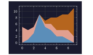
let xs = [0, 1, 2, 3, 4, 5, 6, 7, 8, 9]
let y1 = [0, 1, 3, 9, 5, 4, 2, 2, 1, 0]
let y2 = [5, 3, 2, 0, 1, 2, 2, 2, 3, 2]
let y3 = [0, 0, 0, 0, 1, 2, 4, 5, 5, 9]

diagram(
    stacked_area(xs, y1, y2, y3),
    theme = "moon"
)
Themes
Kleis supports Lilaq’s built-in themes:
| Theme | Description |
|---|---|
schoolbook | Math textbook style with axes at origin |
moon | Dark theme for presentations |
ocean | Blue-tinted theme |
misty | Soft, muted colors |
skyline | Clean, modern look |
diagram(
    plot(xs, ys),
    theme = "moon"
)
Axis Customization
| Option | Description | Example |
|---|---|---|
xlim, ylim | Axis limits | xlim = [-6.28, 6.28] |
xaxis_tick_unit | Tick spacing unit | xaxis_tick_unit = 3.14159 |
xaxis_tick_suffix | Tick label suffix | xaxis_tick_suffix = "pi" |
xaxis_tick_rotate | Rotate labels | xaxis_tick_rotate = -90 |
xaxis_ticks_none | Hide ticks | xaxis_ticks_none = true |
Complete Example Notebook
Cell 1: Import stdlib
import "stdlib/prelude.kleis"
Cell 2: Generate data with linspace
let xs = linspace(0, 6.28, 50)
let ys = list_map(lambda x . sin(x), xs)
Cell 3: Plot with theme
diagram(
    plot(xs, ys, color = "blue", stroke = "2pt"),
    title = "Sine Wave",
    xlabel = "x",
    ylabel = "sin(x)",
    theme = "moon"
)
Logarithmic Scales
For exponential or power-law data, use logarithmic scales:
// Semi-log plot (linear x, logarithmic y)
diagram(
    plot([0, 1, 2, 3, 4], [1, 10, 100, 1000, 10000]),
    title = "Exponential Growth",
    yscale = "log"   // "linear", "log", or "symlog"
)

// Log-log plot (both axes logarithmic)
diagram(
    plot([1, 10, 100, 1000], [1, 100, 10000, 1000000]),
    title = "Power Law",
    xscale = "log",
    yscale = "log"
)
Available scales:
"linear"- Default linear scale"log"- Logarithmic scale (base 10)"symlog"- Symmetric log (linear near 0, log elsewhere; handles negative values)
Next Steps
- Learn to create PDFs, theses, and papers: Document Generation
- Explore the REPL chapter for more interactive features
- See Matrices for symbolic matrix operations
- Check Z3 Verification for formal proofs