The Kleis Manual
“Mathematics is the language with which God has written the universe.” — Galileo Galilei
Welcome to The Kleis Manual, the official guide to the Kleis mathematical specification language.
What is Kleis?
Kleis is a structure-oriented mathematical formalization language with Z3 verification and LAPACK numerics.
Philosophy: Structures — the foundation of everything.
| Metric | Value |
|---|---|
| Grammar | Fully implemented |
| Tests | 1,762 Rust unit tests |
| Examples | 71 Kleis files across 15+ domains |
| Built-in Functions | 100+ (including LAPACK numerical operations) |
Core Capabilities
- 🏗️ Structure-first design — define mathematical objects by their axioms, not just their data
- ✅ Z3 verification — prove properties with SMT solving
- 🔢 LAPACK numerics — eigenvalues, SVD, matrix exponentials, and more
- 📐 Symbolic mathematics — work with expressions, not just numbers
- 🔬 Scientific computing — differential geometry, tensor calculus, control systems
- 🔄 Turing complete — a full programming language, not just notation
Computational Universality: Kleis is Turing complete. This was demonstrated by implementing a complete LISP interpreter in Kleis (see Appendix: LISP Interpreter). The combination of algebraic data types, pattern matching, and recursion enables arbitrary computation.
Domain Coverage
Kleis has been used to formalize:
| Domain | Examples |
|---|---|
| Mathematics | Differential forms, tensor algebra, complex analysis, number theory |
| Physics | Dimensional analysis, quantum entanglement, orbital mechanics |
| Control Systems | LQG controllers, eigenvalue analysis, state-space models |
| Ontology | Projected Ontology Theory, spacetime types |
| Protocols | IPv4 packets, IP routing, stop-and-wait ARQ |
| Authorization | OAuth2 scopes, Google Zanzibar |
| Formal Methods | Petri nets, mutex verification |
| Games | Chess, Contract Bridge, Sudoku |
Who is This For?
Kleis is for anyone who thinks in terms of structures and axioms:
- Mathematicians — formalize theorems, verify properties, explore number theory
- Physicists — tensor algebra, differential geometry, dimensional analysis
- Engineers — control systems, protocol specifications, verified designs
- Security architects — authorization policies (Zanzibar, OAuth2)
- Researchers — formalize new theories with Z3 verification
- Functional programmers — if you enjoy Haskell or ML, you’ll feel at home
If you’ve ever wished you could prove your specifications are consistent, Kleis is for you.
Why Kleis Now?
Modern systems demand formal verification:
| Challenge | How Kleis Helps |
|---|---|
| Security & Compliance | Machine-checkable proofs for audit trails across sectors |
| Complex Systems | Verify rules across IoT, enterprise, and distributed systems |
| AI-Generated Content | Verify AI outputs against formal specifications |
Universal verification — same rigor for mathematics, business rules, and beyond.
How to Read This Guide
Each chapter builds on the previous ones. We start with the basics:
- Starting Out — expressions, operators, basic syntax
- Types — naming and composing structures
- Functions — operations with laws
Then we explore core concepts:
- Algebraic Types — data definitions and constructors
- Pattern Matching — elegant case analysis
- Let Bindings — local definitions
- Quantifiers and Logic — ∀, ∃, and logical operators
- Conditionals — if-then-else
And advanced features:
- Structures — the foundation of everything
- Implements — structure implementations
- Z3 Verification — proving things with SMT
Philosophy: In Kleis, structures define what things are through their operations and axioms. Types are names for structures. A metric tensor isn’t “a 2D array” — it’s “something satisfying metric axioms.”
A Taste of Kleis
Here’s what Kleis looks like:
// Define a function
define square(x) = x * x

// With type annotation
define double(x : ℝ) : ℝ = x + x

// Create a structure with axioms
structure Group(G) {
    operation e : G                    // identity
    operation inv : G → G              // inverse
    operation mul : G × G → G          // multiplication

    axiom left_identity : ∀ x : G . mul(e, x) = x
    axiom left_inverse : ∀ x : G . mul(inv(x), x) = e
}

// Numerical computation
example "eigenvalues" {
    let A = Matrix([[1, 2], [3, 4]]) in
    out(eigenvalues(A))  // Pretty-printed output
}
Getting Started
Ready? Let’s dive in!
→ Start with Chapter 1: Starting Out
Starting Out
Your First Kleis Expression
The simplest things in Kleis are expressions. An expression is anything that has a value:
define answer = 42              // A number
define pi_approx = 3.14159      // A decimal
define sum(x, y) = x + y        // An arithmetic expression
define angle_sin(θ) = sin(θ)    // A function call
The REPL
The easiest way to experiment with Kleis is the REPL (Read-Eval-Print Loop):
$ cargo run --bin repl
🧮 Kleis REPL v0.1.0
   Type :help for commands, :quit to exit

λ> 2 + 2
2 + 2

λ>  let x = 5 in x * x
times(5, 5)
Basic Arithmetic
Kleis supports the usual arithmetic operations:
define add_example = 2 + 3       // Addition: 5
define sub_example = 10 - 4      // Subtraction: 6
define mul_example = 3 * 7       // Multiplication: 21
define div_example = 15 / 3      // Division: 5
define pow_example = 2 ^ 10      // Exponentiation: 1024
Variables and Definitions
Use define to create named values:
define pi = 3.14159
define e = 2.71828
define golden_ratio = (1 + sqrt(5)) / 2
Functions are defined similarly:
define square(x) = x * x
define cube(x) = x * x * x
define area_circle(r) = pi * r^2
Comments
Kleis uses C-style comments:
// This is a single-line comment
define x = 42  // Inline comment

/*
   Multi-line comments
   use slash-star syntax
*/
Unicode Support
Kleis embraces mathematical notation with full Unicode support:
// Greek letters
define α = 0.5
define β = 1.0
define θ = π / 4

// Mathematical symbols in axioms
axiom reflexivity : ∀(x : ℝ). x = x           // Universal quantifier
axiom positive_exists : ∃(y : ℝ). y > 0       // Existential quantifier
You can use ASCII alternatives too:
| Unicode | ASCII Alternative |
|---|---|
∀ | forall |
∃ | exists |
→ | -> |
What’s Next?
Now that you can write basic expressions, let’s learn about the type system!
Types and Values
Why Types Matter
Types are the foundation of Kleis. Every expression has a type, and the type system catches errors before they become problems.
define answer = 42                // 42 is an integer
define pi_val = 3.14              // 3.14 is a real number
define flag = True                // True is a boolean
Built-in Types
Numeric Types
| Type | Unicode | Full Name | ASCII | Examples |
|---|---|---|---|---|
| Natural | ℕ | Nat | N | 0, 42, 100 |
| Integer | ℤ | Int | Z | -5, 0, 17 |
| Rational | ℚ | Rational | Q | rational(1, 2), rational(3, 4) |
| Real | ℝ | Real or Scalar | R | 3.14, -2.5, √2 |
| Complex | ℂ | Complex | C | 3 + 4i, i |
Other Basic Types
| Type | Unicode | Full Name | Values |
|---|---|---|---|
| Boolean | 𝔹 | Bool | True, False |
| String | — | String | "hello", "world" |
| Unit | — | Unit | () |
Parameterized Primitive Types
| Type | Syntax | Description |
|---|---|---|
| Bit-Vector | BitVec(n) | n-bit binary vector (e.g., BitVec(8), BitVec(32)) |
| Set | Set(T) | Set of elements of type T (e.g., Set(ℤ), Set(ℝ)) |
// Boolean values
define flag = True
define not_flag = False

// Boolean in quantified expressions (inside structures)
structure BoolExamples {
    axiom reflexive_unicode : ∀(p : 𝔹). p = p
    axiom reflexive_full    : ∀(q : Bool). q = q
}
The Unit Type
The Unit type represents “no meaningful value” — like void in C or () in Rust/Haskell. It has exactly one value: ().
When to use Unit:
- Result types that can fail but return nothing on success:
// A validation that succeeds with () or fails with an error message
data ValidationResult = Ok(Unit) | Err(String)

define validate_positive(x : ℝ) : ValidationResult =
    if x > 0 then Ok(()) else Err("must be positive")
- Optional values where presence matters, not content:
// Option type - Some(value) or None
data Option(T) = Some(T) | None

// A flag that's either set or not (no associated value)
define flag_set : Option(Unit) = Some(())
define flag_unset : Option(Unit) = None
- Proof terms with no computational content:
// A theorem that x = x (the proof itself carries no data)
structure Reflexivity {
    axiom refl : ∀(x : ℝ). x = x
}
// The "witness" of this axiom would have type Unit
Type Annotations
You can explicitly annotate types with ::
// Variable annotation
define typed_let = let x : ℝ = 3.14 in x * 2

// Function parameter and return types
define f(x : ℝ) : ℝ = x * x

// Expression-level annotation (ascription)
define sum_typed(a, b) = (a + b) : ℝ
Type Aliases
Type aliases give a new name to an existing type, making your code more readable and self-documenting.
The type Keyword
type Probability = ℝ
type Temperature = ℝ
type Velocity = ℝ
Now you can use Probability instead of ℝ to make your intent clear:
define coin_flip : Probability = 0.5
define boiling_point : Temperature = 100.0
Why Use Type Aliases?
- Readability —
Probabilityis clearer thanℝ - Documentation — the type name explains what the value represents
- Refactoring — change the underlying type in one place
Function Type Aliases
Type aliases are especially useful for complex function types:
type RealFunction = ℝ → ℝ
type BinaryOp = ℝ → ℝ → ℝ
type Predicate = ℝ → Bool
Now instead of writing (ℝ → ℝ) → ℝ, you can write:
type Integrator = RealFunction → ℝ
Parameterized Type Aliases
Type aliases can have parameters:
type Pair(T) = T → T → T
type Endomorphism(T) = T → T
Aliases for Data Types and Structures
Type aliases work with user-defined types too:
// Alias for a data type (sum type)
data Option(T) = Some(value : T) | None
type MaybeInt = Option(ℤ)
type MaybeString = Option(String)

// Alias for a structure (product type)
structure Point {
    x : ℝ
    y : ℝ
}
type Coordinate = Point

// Alias for nested ADTs
data Result(T, E) = Ok(value : T) | Err(error : E)
type IntResult = Result(ℤ, String)
Note: Type aliases create a synonym —
Probabilityandℝare interchangeable. They don’t create a distinct new type.
Function Types
Functions have types too! The notation A → B means “a function from A to B”:
// square takes a Real and returns a Real
define square(x : ℝ) : ℝ = x * x
// Type: ℝ → ℝ

// add takes two Reals and returns a Real
define add(x : ℝ, y : ℝ) : ℝ = x + y
// Type: ℝ × ℝ → ℝ (or equivalently: ℝ → ℝ → ℝ)
Higher-Order Function Types
Functions can take other functions as arguments or return functions. These are called higher-order functions:
// A function that takes a function as an argument
define apply_twice(f : ℝ → ℝ, x : ℝ) : ℝ = f(f(x))
// Type: (ℝ → ℝ) × ℝ → ℝ

// A function that returns a function
define make_adder(n : ℝ) : ℝ → ℝ = ???
// Type: ℝ → (ℝ → ℝ)
The parentheses matter! Compare:
(ℝ → ℝ) → ℝ— takes a function, returns a numberℝ → (ℝ → ℝ)— takes a number, returns a functionℝ → ℝ → ℝ— curried function (associates right:ℝ → (ℝ → ℝ))
Function Type Examples
| Type | Meaning |
|---|---|
ℝ → ℝ | Function from real to real |
ℝ → ℝ → ℝ | Curried binary function |
(ℝ → ℝ) → ℝ | Takes a function, returns a value (e.g., definite integral) |
ℝ → (ℝ → ℝ) | Returns a function (function factory) |
(ℝ → ℝ) → (ℝ → ℝ) | Function transformer (e.g., derivative operator) |
Set Types
Kleis provides a built-in Set(T) type backed by Z3’s native set theory. Sets are unordered collections of unique elements:
// Declare a set type
define S : Set(ℤ)

// Set operations (see stdlib/sets.kleis for full structure)
in_set(x, S)              // Membership: x ∈ S → Bool
union(A, B)               // Union: A ∪ B → Set(T)
intersect(A, B)           // Intersection: A ∩ B → Set(T)
difference(A, B)          // Difference: A \ B → Set(T)
complement(A)             // Complement: ᶜA → Set(T)
subset(A, B)              // Subset test: A ⊆ B → Bool
insert(x, S)              // Add element: S ∪ {x} → Set(T)
remove(x, S)              // Remove element: S \ {x} → Set(T)
singleton(x)              // Singleton set: {x} → Set(T)
empty_set                 // Empty set: ∅
Set Theory Axioms
Sets come with a complete axiomatization (see stdlib/sets.kleis):
structure SetTheory(T) {
    // Core operations
    operation in_set : T → Set(T) → Bool
    operation union : Set(T) → Set(T) → Set(T)
    operation intersect : Set(T) → Set(T) → Set(T)
    element empty_set : Set(T)

    // Extensionality: sets are equal iff they have the same elements
    axiom extensionality: ∀(A B : Set(T)).
        (∀(x : T). in_set(x, A) ↔ in_set(x, B)) → A = B

    // Union definition
    axiom union_def: ∀(A B : Set(T), x : T).
        in_set(x, union(A, B)) ↔ (in_set(x, A) ∨ in_set(x, B))

    // De Morgan's laws
    axiom de_morgan_union: ∀(A B : Set(T)).
        complement(union(A, B)) = intersect(complement(A), complement(B))
}
Using Sets in Verification
Sets are particularly useful for specifying properties involving collections:
structure MetricSpace(X) {
    operation d : X → X → ℝ
    operation ball : X → ℝ → Set(X)

    // Open ball definition
    axiom ball_def: ∀(center : X, radius : ℝ, x : X).
        in_set(x, ball(center, radius)) ↔ d(x, center) < radius
}
Parametric Types
Types can have parameters:
// Parametric type examples:
List(ℤ)           // List of integers
Matrix(3, 3, ℝ)   // 3×3 matrix of reals
Vector(4)         // 4-dimensional vector
Set(ℝ)            // Set of real numbers
Dimension Expressions
When working with parameterized types like Matrix(m, n, ℝ), the dimension parameters are not just simple numbers — they can be dimension expressions. This enables type-safe operations where dimensions depend on each other.
Supported Dimension Expressions
| Category | Operators | Examples |
|---|---|---|
| Arithmetic | +, -, *, / | n+1, 2*n, n/2 |
| Power | ^ | n^2, 2^k |
| Grouping | ( ) | (n+1)*2 |
| Functions | min, max | min(m, n) |
Why Dimension Expressions Matter
Consider the realification functor from control theory, which embeds a complex n×n matrix into a real 2n×2n matrix:
// Complex matrix represented as (real_part, imag_part)
type ComplexMatrix(m: Nat, n: Nat) = (Matrix(m, n, ℝ), Matrix(m, n, ℝ))

// Realification: embed C^(n×n) into R^(2n×2n)
structure Realification(n: Nat) {
    operation realify : ComplexMatrix(n, n) → Matrix(2*n, 2*n, ℝ)
    operation complexify : Matrix(2*n, 2*n, ℝ) → ComplexMatrix(n, n)
}
The 2*n dimension expression captures the invariant that the output dimension is always twice the input dimension.
How Dimension Unification Works
When Kleis type-checks your code, it must verify that dimension expressions match. This uses a built-in dimension solver that can handle common arithmetic constraints.
What the Solver Can Unify
| Expression 1 | Expression 2 | Result |
|---|---|---|
2*n | 2*n | ✅ Structurally equal |
2*n | 6 | ✅ Solved: n = 3 |
n + 1 | 5 | ✅ Solved: n = 4 |
n^2 | 9 | ✅ Solved: n = 3 |
2^k | 8 | ✅ Solved: k = 3 |
What the Solver Rejects
| Expression 1 | Expression 2 | Result |
|---|---|---|
2*n | n | ❌ Different structure (unless n = 0) |
n + 1 | n | ❌ Different structure |
n*m | 6 | ⚠️ Underdetermined |
Examples in Practice
Matrix multiplication requires matching inner dimensions:
// Matrix(m, n) × Matrix(n, p) → Matrix(m, p)
structure MatrixMultiply(m: Nat, n: Nat, p: Nat) {
    operation matmul : Matrix(m, n, ℝ) → Matrix(n, p, ℝ) → Matrix(m, p, ℝ)
}
The n dimension must match on both sides — the solver verifies this.
SVD decomposition produces matrices with min(m, n) dimensions:
// Illustrative — tuple return types in structures are aspirational
structure SVD(m: Nat, n: Nat) {
    // A = U * Σ * Vᵀ where Σ is min(m,n) × min(m,n)
    operation svd : Matrix(m, n, ℝ) →
        (Matrix(m, min(m,n), ℝ), Matrix(min(m,n), min(m,n), ℝ), Matrix(min(m,n), n, ℝ))
}
Simplification
The dimension solver simplifies expressions before comparing them:
| Expression | Simplified |
|---|---|
0 + n | n |
1 * n | n |
n^1 | n |
n^0 | 1 |
2 * 3 | 6 |
This means Matrix(1*n, n+0, ℝ) correctly unifies with Matrix(n, n, ℝ).
Design Philosophy
The dimension solver is deliberately bounded:
- It handles practical cases (linear arithmetic, powers, min/max)
- It fails clearly on complex constraints it cannot solve
- It doesn’t require external dependencies (no SMT solver needed for type checking)
If you need more advanced constraint solving, use the :verify command with Z3 at the value level.
Type Inference
Kleis often infers types automatically:
define double(x) = x + x
// Kleis infers: double : ℝ → ℝ (or more general)

define square_five = let y = 5 in y * y
// Kleis infers: y : ℤ
But explicit types make code clearer and catch errors earlier!
The Type Hierarchy
                    Any
         /     |      \       \
     Scalar  String  Collection  Set(T)
     /    \              |
    ℂ    Bool          List
    |                 /    \
    ℝ            Vector   Matrix
    |
    ℚ
    |
    ℤ
    |
    ℕ
Note: ℕ ⊂ ℤ ⊂ ℚ ⊂ ℝ ⊂ ℂ (naturals ⊂ integers ⊂ rationals ⊂ reals ⊂ complex)
Set(T) is parameterized by its element type. Set(ℤ) is a set of integers, Set(ℝ) is a set of reals, etc.
Type Promotion (Embedding)
When you mix numeric types in an expression, Kleis automatically promotes the smaller type to the larger one. This is called type embedding, not subtyping.
Embedding vs Subtyping
| Concept | Meaning | Kleis Approach |
|---|---|---|
| Subtyping | S can be used anywhere T is expected, with identical behavior | Not used |
| Embedding | S can be converted to T via an explicit lift function | ✓ Used |
The difference is subtle but important:
// Embedding: Integer 3 is lifted to Rational before the operation
rational(1, 2) + 3
// Becomes: rational_add(rational(1, 2), lift(3))
// Result: rational(7, 2) — exact!
How Promotion Works
- Type inference determines the result type (the “common supertype”)
- Lifting converts arguments to the target type
- Operation executes at the target type
Int + Rational
    ↓ find common supertype
  Rational
    ↓ lift Int to Rational
  lift(Int) + Rational
    ↓ execute operation
  rational_add(Rational, Rational)
    ↓
  Rational result
The Promotes Structure
Type promotion is defined by the Promotes(From, To) structure:
structure Promotes(From, To) {
  operation lift : From → To
}

// Built-in promotions
implements Promotes(ℕ, ℤ) { operation lift = builtin_nat_to_int }
implements Promotes(ℤ, ℚ) { operation lift = builtin_int_to_rational }
implements Promotes(ℚ, ℝ) { operation lift = builtin_rational_to_real }
implements Promotes(ℝ, ℂ) { operation lift = builtin_real_to_complex }
Defining Your Own Promotions
You can define promotions for your own types. Unlike built-in types (which use builtin_* functions), you must write the conversion function yourself:
data Percentage = Pct(value: ℝ)

// Step 1: Define the conversion function
define pct_to_real(p: Percentage) : ℝ =
  match p { Pct(v) => divide(v, 100) }

// Step 2: Register the promotion, referencing YOUR function
implements Promotes(Percentage, ℝ) {
  operation lift = pct_to_real   // References the function above
}
Now this works in the REPL:
λ> :eval 0.5 + pct_to_real(Pct(25))
✅ 0.75
Key difference from built-in types:
| Type | Lift Implementation |
|---|---|
Built-in (ℤ → ℚ) | operation lift = builtin_int_to_rational (provided by Kleis) |
| User-defined | operation lift = your_function (you must define it) |
Important: For concrete execution (
:eval), you must provide an actualdefinefor the lift function. Without it:
:verify(symbolic) — Works (Z3 treatsliftas uninterpreted):eval(concrete) — Fails (“function not found”)
Precision Considerations
Warning: Promotion can lose precision!
| Promotion | Precision |
|---|---|
ℕ → ℤ | ✓ Exact (integers contain all naturals) |
ℤ → ℚ | ✓ Exact (rationals contain all integers) |
ℚ → ℝ | ⚠️ May lose precision (floating-point approximation) |
ℝ → ℂ | ✓ Exact (complex with zero imaginary part) |
// Exact in Rational
define third : ℚ = rational(1, 3)  // Exactly 1/3

// Approximate in Real (floating-point)
define approx : ℝ = 1.0 / 3.0      // 0.333333...

// If you promote:
define promoted = third + 0.5      // third lifted to ℝ, loses exactness!
Recommendation: When precision matters, be explicit about types:
// Keep it in Rational for exact arithmetic
define exact_sum : ℚ = rational(1, 3) + rational(1, 6)  // Exactly 1/2

// Or use type annotations to prevent accidental promotion
define result(x : ℚ, y : ℚ) : ℚ = x + y
No LSP Violations
Because Kleis uses embedding (not subtyping), operations are always resolved at the target type after lifting. This means:
Int + Intuses integer additionInt + Rationallifts the Int first, then uses rational addition- You never accidentally get integer truncation when you expected rational division
5 / 3           // Integer division → 1 (if both are Int)
rational(5, 1) / rational(3, 1)   // Rational division → 5/3 (exact)
What’s Next?
Types are the foundation. Now let’s see how to define functions!
Functions
Defining Functions
Functions are defined with define:
define square(x) = x * x
define cube(x) = x * x * x
define add(x, y) = x + y
Functions with Type Annotations
For clarity and safety, add type annotations:
define square(x : ℝ) : ℝ = x * x

define distance(x : ℝ, y : ℝ) : ℝ = sqrt(x^2 + y^2)

define normalize(v : Vector(3)) : Vector(3) = v / magnitude(v)
Multi-Parameter Functions
Functions can take multiple parameters:
define add(x, y) = x + y
define volume_box(l, w, h) = l * w * h
define dot_product(a, b, c, x, y, z) = a*x + b*y + c*z
Recursive Functions
Functions can call themselves:
define factorial(n : ℕ) : ℕ =
    if n = 0 then 1
    else n * factorial(n - 1)

define fibonacci(n : ℕ) : ℕ =
    if n ≤ 1 then n
    else fibonacci(n-1) + fibonacci(n-2)
Built-in Mathematical Functions
Kleis includes standard mathematical functions:
Trigonometric
sin(x)      cos(x)      tan(x)
asin(x)     acos(x)     atan(x)
sinh(x)     cosh(x)     tanh(x)
Exponential and Logarithmic
exp(x)      // e^x
ln(x)       // natural log
log(x)      // base-10 log
log(b, x)   // log base b of x
Other
sqrt(x)     // square root
abs(x)      // absolute value
floor(x)    // round down
ceil(x)     // round up
min(x, y)   // minimum
max(x, y)   // maximum
Lambda Expressions (Anonymous Functions)
Lambda expressions allow you to create anonymous functions inline:
define square_lambda = λ x . x * x
define increment = lambda x . x + 1
define add_lambda = λ x . λ y . x + y
define square_typed = λ (x : ℝ) . x^2
define curried_add = λ x . λ y . x + y
Lambda expressions are first-class values - you can pass them to functions:
// Pass lambda to higher-order function
define doubled_list = map(λ x . x * 2, [1, 2, 3])

// Or define inline
define result = apply(λ x . x + 1, 5)
Higher-Order Functions
Functions can take functions as arguments:
// Apply a function twice
define apply_twice(f, x) = f(f(x))

// Example usage:
define inc(x) = x + 1
define result = apply_twice(inc, 5)   // Result: 7
Partial Application and Currying
With lambda expressions, you can create curried functions:
// Curried addition
define add = λ x . λ y . x + y

// Partial application creates specialized functions
define add5 = add(5)           // λ y . 5 + y
define eight = add5(3)         // Result: 8
Named Arguments (v0.96)
For plotting and numeric functions, Kleis supports named arguments (keyword arguments):
// Named arguments come after positional arguments
diagram(
    bar(xs, ys, offset = -0.2, width = 0.4, label = "Data"),
    plot(x, y, color = "blue", yerr = errors),
    width = 10,
    height = 7,
    title = "My Chart"
)
Syntax
Named arguments use = (not ==) and must come after all positional arguments:
// ✅ Valid: positional first, then named
f(a, b, x = 1, y = 2)

// ✅ Valid: all named
f(x = 1, y = 2)

// ❌ Invalid: positional after named
f(x = 1, a, b)      // Error!
Parser Transformation
Named arguments are syntactic sugar. The parser transforms them into a record expression:
// You write:
bar(xs, ys, offset = -0.2, width = 0.4)

// Parser produces:
bar(xs, ys, record(
    field("offset", -0.2),
    field("width", 0.4)
))
Limitations: Numeric Only
Important: Named arguments are designed for concrete numeric computation (plotting, configuration). They cannot be used in:
structuredefinitionsaxiomdeclarationsimplementsblocks- Z3 verification proofs
// ❌ Does NOT work in axioms
structure Bad {
    axiom wrong: f(x = 1)  // ERROR: named args not for axioms
}

// ✅ Works in plotting/computation
let xs = [0, 1, 2, 3]
let ys = [10, 20, 15, 25]
diagram(bar(xs, ys, color = "blue"))
Why This Design?
Named arguments are opaque to the type system:
- Type inference sees
recordas an opaque type - Unification doesn’t look inside records
- Z3 never receives record expressions
- Built-in functions consume records at runtime
This ensures named arguments don’t interfere with symbolic mathematics while providing convenient syntax for plotting and configuration.
What’s Next?
Learn about algebraic data types for structured data!
Algebraic Data Types
What Are ADTs?
Algebraic Data Types (ADTs) let you define custom data structures by combining simpler types. There are two main kinds:
- Product types — “this AND that” (records, tuples)
- Sum types — “this OR that” (variants, enums)
Product Types
A product type combines multiple values:
// A point has an x AND a y
structure Point {
    x : ℝ
    y : ℝ
}

// A person has a name AND an age
structure Person {
    name : String
    age : ℕ
}
Sum Types (Variants)
A sum type represents alternatives — a value that can be one of several different forms.
The data Keyword
In Kleis, you define sum types using the data keyword:
data TypeName = Constructor1 | Constructor2 | Constructor3
Syntax breakdown:
data— keyword that introduces a new type definitionTypeName— the name of your new type (starts with uppercase)=— separates the type name from its constructorsConstructor1,Constructor2, etc. — the possible variants (each starts with uppercase)|— read as “or” — separates the alternatives
Constructors with Data
Constructors can carry data (fields):
data TypeName = Constructor1(field1 : Type1) | Constructor2(field2 : Type2, field3 : Type3)
Each constructor acts like a function that creates a value of the type.
Parameterized Types (Generics)
Types can have parameters, making them work with any type:
data Option(T) = Some(value : T) | None
Here T is a type parameter. You can use Option(ℕ) for optional natural numbers, Option(String) for optional strings, etc. The type is generic — it works for any T.
Examples
// A shape is a Circle OR a Rectangle OR a Triangle
data Shape = Circle(radius : ℝ) | Rectangle(width : ℝ, height : ℝ) | Triangle(a : ℝ, b : ℝ, c : ℝ)

// An optional value is Some(value) OR None
data Option(T) = Some(value : T) | None

// A result is Ok(value) OR Err(message)
data Result(T, E) = Ok(value : T) | Err(error : E)
Pattern Matching with ADTs
ADTs shine with pattern matching:
define area(shape) =
    match shape {
        Circle(r) => π * r^2
        Rectangle(w, h) => w * h
        Triangle(a, b, c) =>
            let s = (a + b + c) / 2 in
            sqrt(s * (s-a) * (s-b) * (s-c))
    }
Recursive Types
Types can refer to themselves:
// A list is either empty (Nil) or a value followed by another list (Cons)
data List(T) {
    Nil
    Cons(head : T, tail : List(T))
}

// A binary tree
data Tree(T) {
    Leaf(value : T)
    Node(left : Tree(T), value : T, right : Tree(T))
}
The Mathematical Perspective
Why “algebraic”?
- Product types correspond to multiplication:
Point = ℝ × ℝ - Sum types correspond to addition:
Option(T) = T + 1
The number of possible values follows algebra:
Boolhas 2 valuesBool × Boolhas 2 × 2 = 4 valuesBool + Boolhas 2 + 2 = 4 values
Practical Example: Expression Trees
ADTs are perfect for representing mathematical expressions:
data Expression =
    ENumber(value : ℝ)
  | EVariable(name : String)
  | EOperation(name : String, args : List(Expression))

// Helper constructors for cleaner syntax
define num(n) = ENumber(n)
define var(x) = EVariable(x)
define e_add(a, b) = EOperation("plus", Cons(a, Cons(b, Nil)))
define e_mul(a, b) = EOperation("times", Cons(a, Cons(b, Nil)))
define e_neg(a) = EOperation("neg", Cons(a, Nil))

define eval_expr(expr, env) =
    match expr {
        ENumber(v) => v
        EVariable(name) => lookup(env, name)
        EOperation("plus", Cons(l, Cons(r, Nil))) =>
            eval_expr(l, env) + eval_expr(r, env)
        EOperation("times", Cons(l, Cons(r, Nil))) =>
            eval_expr(l, env) * eval_expr(r, env)
        EOperation("neg", Cons(e, Nil)) =>
            -eval_expr(e, env)
        _ => 0
    }
What’s Next?
Let’s dive deeper into pattern matching!
Pattern Matching
The Power of Match
Pattern matching is one of Kleis’s most powerful features. It lets you destructure data and handle different cases elegantly:
define describe(n) =
    match n {
        0 => 0
        1 => 1
        _ => 2
    }
Basic Patterns
Literal Patterns
Match exact values:
define describe_literal(x) =
    match x {
        0 => "zero"
        1 => "one"
        42 => "the answer"
        _ => "something else"
    }
Variable Patterns
Bind matched values to names:
define sum_point(point) =
    match point {
        Point(x, y) => x + y
    }
Wildcard Pattern
The underscore _ matches anything:
define describe_pair(pair) =
    match pair {
        (_, 0) => "second is zero"
        (0, _) => "first is zero"
        _ => "neither is zero"
    }
Nested Patterns
Patterns can be nested arbitrarily:
define sum_tree(tree) =
    match tree {
        Leaf(v) => v
        Node(Leaf(l), v, Leaf(r)) => l + v + r
        Node(left, v, right) => v + sum_tree(left) + sum_tree(right)
    }
Guards
Add conditions to patterns with if:
define sign(n) =
    match n {
        x if x < 0 => "negative"
        x if x > 0 => "positive"
        _ => "zero"
    }
As-Patterns
Bind the whole match while also destructuring:
define filter_head(list) =
    match list {
        Cons(h, t) as whole =>
            if h > 10 then whole
            else t
        Nil => Nil
    }
Pattern Matching in Let
Destructure directly in let bindings:
define distance_squared(origin) =
    let Point(x, y) = origin in x^2 + y^2

define sum_first_two(triple) =
    let (first, second, _) = triple in first + second
Pattern Matching in Function Parameters
With lambda expressions now available, you can combine them with match:
// Pattern matching with lambdas
define fst = λ pair . match pair { (a, _) => a }
define snd = λ pair . match pair { (_, b) => b }
Alternative workaround:
define fst(pair) =
    match pair {
        (a, _) => a
    }
Exhaustiveness
Kleis checks that your patterns cover all cases:
// ⚠️ Warning: non-exhaustive patterns
define incomplete(opt) =
    match opt {
        Some(x) => x
    }

// ✓ Complete
define complete(opt) =
    match opt {
        Some(x) => x
        None => 0
    }
Real-World Example: Symbolic Differentiation
Pattern matching makes symbolic math elegant:
define diff(expr, var) =
    match expr {
        Const(_) => Const(0)

        Var(name) =>
            if name = var then Const(1)
            else Const(0)

        Add(f, g) =>
            Add(diff(f, var), diff(g, var))

        Mul(f, g) =>
            Add(Mul(diff(f, var), g),
                Mul(f, diff(g, var)))

        Neg(f) =>
            Neg(diff(f, var))
    }
Note: This
difffunction computes derivatives by pattern matching on expression trees. Kleis also providesD(f, x)andDt(f, x)operations instdlib/calculus.kleisfor verifying derivative properties with Z3. See Applications: Symbolic Differentiation for a detailed comparison.
What’s Next?
Learn about let bindings for local definitions!
Let Bindings
Introduction
Let bindings introduce local variables with limited scope. They’re essential for breaking complex expressions into readable parts.
define square_five = let x = 5 in x * x
// Result: 25
Basic Syntax
let <name> = <value> in <body>
The variable name is only visible within body:
define circle_area = let radius = 10 in π * radius^2
// Result: 314.159...
// 'radius' is not visible outside the let binding
With Type Annotations
Add explicit types for clarity:
define typed_example1 = let x : ℝ = 3.14 in x * 2
define typed_example2 = let n : ℕ = 42 in factorial(n)
define typed_example3 = let v : Vector(3) = [1, 2, 3] in magnitude(v)
Nested Let Bindings
Chain multiple bindings:
define nested_example =
    let x = 5 in
    let y = 3 in
    let z = x + y in
        x * y * z
// Result: 5 * 3 * 8 = 120
Shadowing
Inner bindings can shadow outer ones:
define shadowing_example =
    let x = 1 in
    let x = x + 1 in
    let x = x * 2 in
        x
// Result: 4  (not 1!)
Each let creates a new scope where x is rebound.
Pure Substitution Semantics
In Kleis, let x = e in body is equivalent to substituting e for x in body:
define substitution_demo = let x = 5 in x + x
// is the same as:
define substitution_result = 5 + 5
This is pure functional semantics — no mutation, no side effects.
Practical Examples
Quadratic Formula
define quadratic_roots(a, b, c) =
    let discriminant = b^2 - 4*a*c in
    let sqrt_d = sqrt(discriminant) in
    let denom = 2 * a in
        ((-b + sqrt_d) / denom, (-b - sqrt_d) / denom)
Heron’s Formula
define triangle_area(a, b, c) =
    let s = (a + b + c) / 2 in
        sqrt(s * (s - a) * (s - b) * (s - c))
Complex Calculations
define schwarzschild_metric(r, M) =
    let rs = 2 * G * M / c^2 in
    let factor = 1 - rs / r in
        -c^2 * factor
Let vs Define
define | let ... in |
|---|---|
| Top-level, global | Local scope only |
| Named function/constant | Temporary binding |
| Visible everywhere | Visible only in body |
// Global constant
define pi = 3.14159

// Local temporary in a function
define circumference(radius) = let two_pi = 2 * pi in two_pi * radius
What’s Next?
Learn about quantifiers and logic!
Quantifiers and Logic
Universal Quantifier (∀)
The universal quantifier expresses “for all”:
// Quantified propositions (used inside axioms)
axiom reflexivity : ∀(x : ℝ). x = x
axiom additive_identity : ∀(x : ℝ). x + 0 = x
axiom commutative : ∀(x : ℝ)(y : ℝ). x + y = y + x
ASCII alternative: forall x . ...
Existential Quantifier (∃)
The existential quantifier expresses “there exists”:
// Existential quantifiers
axiom positive_exists : ∃(x : ℝ). x > 0
axiom sqrt2_exists : ∃(y : ℝ). y * y = 2
axiom distinct_exists : ∃(x : ℝ)(y : ℝ). x ≠ y
ASCII alternative: exists x . ...
Combining Quantifiers
Build complex statements:
// Every number has a successor
axiom successor : ∀(n : ℕ). ∃(m : ℕ). m = n + 1

// Density of rationals: between any two reals is a rational
axiom density : ∀(x : ℝ)(y : ℝ). x < y → ∃(q : ℚ). x < q ∧ q < y
Logical Connectives
Conjunction (∧ / and)
define in_range(x) = x > 0 ∧ x < 10     // x is between 0 and 10
define false_example = True ∧ False     // False
Disjunction (∨ / or)
define is_binary(x) = x = 0 ∨ x = 1    // x is 0 or 1
define true_example = True ∨ False     // True
Implication (→ / implies)
define positive_square(x) = x > 0 → x * x > 0   // If positive, square is positive
define implication(P, Q) = P → Q                // If P then Q
Negation (¬ / not)
define nonzero(x) = ¬(x = 0)     // x is not zero
define not_true = ¬True          // False
Biconditional (↔ / iff)
define zero_iff_square_zero(x) = x = 0 ↔ x * x = 0 // x is zero iff x² is zero
Type Constraints in Quantifiers
Restrict the domain:
axiom naturals_nonneg : ∀(x : ℕ). x ≥ 0
axiom det_inverse : ∀(M : Matrix(n, n)). det(M * M⁻¹) = 1
The where Clause
Add conditions to quantified variables using the where keyword:
structure Field(F) {
    element zero : F
    element one : F
    operation inverse : F → F

    // Multiplicative inverse only for non-zero elements
    axiom multiplicative_inverse:
        ∀(x : F) where x ≠ zero. inverse(x) * x = one
}
The where clause restricts the domain before the quantified body is evaluated. This is essential for axioms that don’t apply universally.
More examples:
structure Analysis {
    // Division only defined for non-zero denominator
    axiom division: ∀(a : ℝ)(b : ℝ) where b ≠ 0. a / b * b = a

    // Logarithm only for positive numbers
    axiom log_exp: ∀(x : ℝ) where x > 0. exp(log(x)) = x
}
Using Quantifiers in Axioms
Quantifiers are essential in structure axioms:
structure Group(G) {
    e : G                      // Identity element
    operation mul : G × G → G
    operation inv : G → G

    axiom identity : ∀(x : G). mul(e, x) = x ∧ mul(x, e) = x
    axiom inverse : ∀(x : G). mul(x, inv(x)) = e
    axiom associative : ∀(x : G)(y : G)(z : G).
        mul(mul(x, y), z) = mul(x, mul(y, z))
}
Nested Quantifiers (Grammar v0.9)
Quantifiers can appear inside logical expressions:
structure Analysis {
    // Quantifier inside conjunction
    axiom bounded_positive: (x > 0) ∧ (∀(y : ℝ). abs(y) <= x)

    // Quantifier inside implication
    axiom dense_rationals: ∀(a b : ℝ). a < b → (∃(q : ℚ). a < q ∧ q < b)

    // Deeply nested quantifiers
    axiom limit_def: ∀(L : ℝ, ε : ℝ). ε > 0 →
        (∃(δ : ℝ). δ > 0 ∧ (∀(x : ℝ). abs(x) < δ → abs(f(x) - L) < ε))
}
Epsilon-Delta Limit Definition
The classic analysis definition now parses correctly:
structure Limits {
    axiom epsilon_delta: ∀(f : ℝ → ℝ, L a : ℝ).
        has_limit(f, a, L) ↔
        (∀(ε : ℝ). ε > 0 → (∃(δ : ℝ). δ > 0 ∧
            (∀(x : ℝ). abs(x - a) < δ → abs(f(x) - L) < ε)))
}
Function Types in Quantifiers (Grammar v0.9)
Quantify over functions using the arrow type:
structure FunctionProperties {
    // Quantify over a function ℝ → ℝ
    axiom continuous: ∀(f : ℝ → ℝ, x : ℝ).
        is_continuous(f, x)

    // Quantify over multiple functions
    axiom composition: ∀(f : ℝ → ℝ, g : ℝ → ℝ).
        compose(f, g) = λ x . f(g(x))

    // Higher-order function types
    axiom curried: ∀(f : ℝ → ℝ → ℝ, a b : ℝ).
        f = f
}
Topology with Function Types
structure Topology {
    axiom continuity: ∀(f : X → Y, V : Set(Y)).
        is_open(V) → is_open(preimage(f, V))

    axiom homeomorphism: ∀(f : X → Y, g : Y → X).
        (∀(x : X). g(f(x)) = x) ∧ (∀(y : Y). f(g(y)) = y) →
        bijective(f)
}
Verification with Z3
Kleis uses Z3 to check quantified statements:
// Z3 can verify this is always true:
axiom add_zero : ∀(x : ℝ). x + 0 = x

// Z3 can find a counterexample for this:
axiom all_positive : ∀(x : ℝ). x > 0
// Z3 finds counterexample: x = -1
Truth Tables
| P | Q | P ∧ Q | P ∨ Q | P → Q | ¬P |
|---|---|---|---|---|---|
| T | T | T | T | T | F |
| T | F | F | T | F | F |
| F | T | F | T | T | T |
| F | F | F | F | T | T |
What’s Next?
Learn about conditional expressions!
Conditionals
If-Then-Else
The basic conditional expression:
if condition then value1 else value2
Examples:
define positive_check(x) = if x > 0 then "positive" else "non-positive"

define factorial(n) = if n = 0 then 1 else n * factorial(n - 1)

define abs(x) = if x ≥ 0 then x else -x
Conditionals Are Expressions
In Kleis, if-then-else is an expression that returns a value:
define doubled_abs(x) =
    let result = if x > 0 then x else -x in
    result * 2

// Both branches must have compatible types!
// if True then 42 else "hello"  // ❌ Type error!
Nested Conditionals
define sign(x) =
    if x > 0 then 1
    else if x < 0 then -1
    else 0

define grade(score) =
    if score ≥ 90 then "A"
    else if score ≥ 80 then "B"
    else if score ≥ 70 then "C"
    else if score ≥ 60 then "D"
    else "F"
Guards vs If-Then-Else
Pattern matching with guards is often cleaner:
// With if-then-else
define classify_if(n) =
    if n < 0 then "negative"
    else if n = 0 then "zero"
    else "positive"

// With pattern matching and guards
define classify_match(n) =
    match n {
        x if x < 0 => "negative"
        0 => "zero"
        _ => "positive"
    }
Piecewise Functions
Mathematicians love piecewise definitions:
// Absolute value
define abs_fn(x) =
    if x ≥ 0 then x else -x

// Heaviside step function
define heaviside(x) =
    if x < 0 then 0
    else if x = 0 then 0.5
    else 1

// Piecewise polynomial
define piecewise_f(x) =
    if x < 0 then x^2
    else if x < 1 then x
    else 2 - x
Boolean Expressions
Conditions can be complex:
define quadrant(x, y) =
    if x > 0 ∧ y > 0 then "first quadrant"
    else if x < 0 ∧ y > 0 then "second quadrant"
    else if x < 0 ∧ y < 0 then "third quadrant"
    else if x > 0 ∧ y < 0 then "fourth quadrant"
    else "on an axis"
Short-Circuit Evaluation
Kleis uses short-circuit evaluation for ∧ and ∨:
// If x = 0, division is never evaluated
define check_ratio(x, y) =
    if x ≠ 0 ∧ y/x > 1 then "big ratio" else "safe"
What’s Next?
Learn about structures for defining mathematical objects!
Structures
What Are Structures?
Structures define mathematical objects with their properties and operations. Think of them as “blueprints” for mathematical concepts.
structure Vector(n : ℕ) {
    // Operations this structure supports
    operation add : Vector(n) → Vector(n)
    operation scale : ℝ → Vector(n)
    operation dot : Vector(n) → ℝ

    // Properties that must hold
    axiom commutative : ∀(u : Vector(n))(v : Vector(n)).
        add(u, v) = add(v, u)
}
Structure Syntax
structure Name(parameters) {
    // Elements (constants)
    element1 : Type1

    // Operations (functions)
    operation op1 : InputType → OutputType

    // Axioms (properties)
    axiom property : logical_statement
}
Structure Members
Structures contain three kinds of members:
The operation Keyword
The operation keyword declares a function that the structure provides:
structure Group(G) {
    operation mul : G × G → G      // Binary operation
    operation inv : G → G          // Unary operation
}
Operations declare the signature (types), not the implementation. The implementation is provided in an implements block (see Chapter 10).
The element Keyword
The element keyword declares a distinguished constant of the structure:
structure Monoid(M) {
    element e : M           // Identity element
    operation mul : M × M → M

    axiom identity : ∀(x : M). mul(e, x) = x
}

structure Field(F) {
    element zero : F        // Additive identity
    element one : F         // Multiplicative identity
}
Elements are constants that satisfy the structure’s axioms. You can also write elements without the element keyword:
structure Ring(R) {
    zero : R    // Same as "element zero : R"
    one : R
}
The axiom Keyword
The axiom keyword declares a property that must hold:
structure Group(G) {
    element e : M
    operation mul : G × G → G
    operation inv : G → G

    axiom identity : ∀(x : G). mul(e, x) = x ∧ mul(x, e) = x
    axiom inverse : ∀(x : G). mul(x, inv(x)) = e
    axiom associative : ∀(x : G)(y : G)(z : G). mul(mul(x, y), z) = mul(x, mul(y, z))
}
Axioms are verified by Z3 when you use implements blocks or run kleis verify.
Example: Complex Numbers
structure Complex {
    re : ℝ  // real part
    im : ℝ  // imaginary part

    operation add : Complex → Complex
    operation mul : Complex → Complex
    operation conj : Complex           // conjugate
    operation mag : ℝ                  // magnitude

    axiom add_commutative : ∀(z : Complex)(w : Complex).
        add(z, w) = add(w, z)

    axiom magnitude_positive : ∀(z : Complex).
        mag(z) ≥ 0

    axiom conj_involution : ∀(z : Complex).
        conj(conj(z)) = z
}
Parametric Structures
Structures can have type parameters:
structure Matrix(m : ℕ, n : ℕ, T) {
    operation transpose : Matrix(n, m, T)
    operation add : Matrix(m, n, T) → Matrix(m, n, T)

    axiom transpose_involution : ∀(A : Matrix(m, n, T)).
        transpose(transpose(A)) = A
}

// Square matrices have more operations
structure SquareMatrix(n : ℕ, T) extends Matrix(n, n, T) {
    operation det : T
    operation trace : T
    operation inv : SquareMatrix(n, T)

    axiom det_mul : ∀(A : SquareMatrix(n, T))(B : SquareMatrix(n, T)).
        det(mul(A, B)) = det(A) * det(B)
}
Nested Structures
Structures can contain other structures. This enables compositional algebra — defining complex structures from simpler parts:
structure Ring(R) {
    // A ring has an additive group
    structure additive : AbelianGroup(R) {
        operation add : R × R → R
        operation negate : R → R
        zero : R
    }

    // And a multiplicative monoid
    structure multiplicative : Monoid(R) {
        operation mul : R × R → R
        one : R
    }

    // With distributivity connecting them
    axiom distributive : ∀(x : R)(y : R)(z : R).
        mul(x, add(y, z)) = add(mul(x, y), mul(x, z))
}
Nested structures can go arbitrarily deep:
structure VectorSpace(V, F) {
    structure vectors : AbelianGroup(V) {
        operation add : V × V → V
        zero : V
    }

    structure scalars : Field(F) {
        operation add : F × F → F
        operation mul : F × F → F
    }

    operation scale : F × V → V
}
When using Z3 verification, axioms from nested structures are automatically available.
The extends Keyword
Structures can extend other structures:
structure Monoid(M) {
    e : M
    operation mul : M × M → M

    axiom identity : ∀(x : M). mul(e, x) = x ∧ mul(x, e) = x
    axiom associative : ∀(x : M)(y : M)(z : M).
        mul(mul(x, y), z) = mul(x, mul(y, z))
}

structure Group(G) extends Monoid(G) {
    operation inv : G → G

    axiom inverse : ∀(x : G). mul(x, inv(x)) = e ∧ mul(inv(x), x) = e
}

structure AbelianGroup(G) extends Group(G) {
    axiom commutative : ∀(x : G)(y : G). mul(x, y) = mul(y, x)
}
The over Keyword
Many mathematical structures are defined “over” a base structure. A vector space is defined over a field, a module over a ring:
// Vector space over a field
structure VectorSpace(V) over Field(F) {
    operation add : V × V → V
    operation scale : F × V → V

    axiom scalar_identity : ∀(v : V). scale(1, v) = v
    axiom distributive : ∀(a : F)(u : V)(v : V).
        scale(a, add(u, v)) = add(scale(a, u), scale(a, v))
}

// Module over a ring (generalization of vector space)
structure Module(M) over Ring(R) {
    operation add : M × M → M
    operation scale : R × M → M
}

// Algebra over a ring
structure Algebra(A) over Ring(R) {
    operation add : A × A → A
    operation scale : R × A → A
    operation mul : A × A → A

    axiom bilinear : ∀(r : R)(a : A)(b : A).
        scale(r, mul(a, b)) = mul(scale(r, a), b)
}
When you use over, Kleis automatically makes the base structure’s axioms available for verification. For example, when verifying VectorSpace axioms, Z3 knows that F satisfies all Field axioms.
Differential Geometry Structures
Kleis shines for differential geometry:
structure Manifold(M, dim : ℕ) {
    operation tangent : M → TangentSpace(M)
    operation metric : M → Tensor(0, 2)

    axiom metric_symmetric : ∀(p : M).
        metric(p) = transpose(metric(p))
}

structure RiemannianManifold(M, dim : ℕ) extends Manifold(M, dim) {
    operation christoffel : M → Tensor(1, 2)
    operation riemann : M → Tensor(1, 3)
    operation ricci : M → Tensor(0, 2)
    operation scalar_curvature : M → ℝ

    // R^a_{bcd} + R^a_{cdb} + R^a_{dbc} = 0
    axiom first_bianchi : ∀(p : M).
        cyclic_sum(riemann(p)) = 0
}
What’s Next?
Learn how to implement structures!
Implements
From Structure to Implementation
A structure declares what operations exist. An implements block provides the actual definitions:
structure Addable(T) {
    operation add : T × T → T
}

implements Addable(ℝ) {
    operation add(x, y) = x + y
}

implements Addable(ℤ) {
    operation add(x, y) = x + y
}
Full Example: Complex Numbers
// Declare the structure
structure Complex {
    re : ℝ
    im : ℝ

    operation add : Complex → Complex
    operation mul : Complex → Complex
    operation conj : Complex
    operation mag : ℝ
}

// Implement the operations
implements Complex {
    operation add(z, w) = builtin_complex_add
    operation mul(z, w) = builtin_complex_mul
    operation conj(z) = builtin_complex_conj
    operation mag(z) = sqrt(z.re^2 + z.im^2)
}
Parametric Implementations
Implement structures with type parameters:
structure Stack(T) {
    operation push : T → Stack(T)
    operation pop : Stack(T)
    operation top : T
    operation empty : Bool
}

implements Stack(ℤ) {
    operation push = builtin_stack_push
    operation pop = builtin_stack_pop
    operation top = builtin_stack_top
    operation empty = builtin_stack_empty
}
Multiple Implementations
The same structure can have multiple implementations:
structure Orderable(T) {
    operation compare : T × T → Ordering
}

// Natural ordering
implements Orderable(ℤ) {
    operation compare = builtin_int_compare
}
Implementing Extended Structures
When a structure extends another, implement all operations:
structure Monoid(M) {
    operation e : M
    operation mul : M × M → M
}

structure Group(G) extends Monoid(G) {
    operation inv : G → G
}

// Must implement both Monoid and Group operations
implements Group(ℤ) {
    operation e = 0
    operation mul(x, y) = x + y
    operation inv(x) = -x
}
Builtin Operations
Some operations can’t be defined in pure Kleis — they need native code. The builtin_ prefix connects Kleis to underlying implementations:
implements Matrix(m, n, ℝ) {
    operation transpose = builtin_transpose
    operation add = builtin_matrix_add
    operation mul = builtin_matrix_mul
}
How Builtins Work
When Kleis sees builtin_foo, it:
- Looks up
fooin the native runtime - Calls the Rust/C/hardware implementation
- Returns the result to Kleis
This enables:
- Performance: Native BLAS for matrix operations
- Hardware access: GPUs, network cards, sensors
- System calls: File I/O, networking, threading
- FFI: Calling existing libraries
The Vision: Hardware as Structures
Imagine:
structure NetworkInterface(N) {
    operation send : Packet → Result(Unit, Error)
    operation receive : Unit → Result(Packet, Error)

    axiom delivery : ∀(p : Packet).
        connected → eventually(delivered(p))
}

implements NetworkInterface(EthernetCard) {
    operation send = builtin_eth_send
    operation receive = builtin_eth_receive
}
The axioms define the contract. The builtins provide the implementation. Z3 can verify that higher-level protocols satisfy their specifications given the hardware axioms.
This is how Kleis becomes a universal verification platform — not just for math, but for any system with verifiable properties.
Verification of Implementations
Kleis + Z3 can verify that implementations satisfy axioms:
structure Monoid(M) {
    e : M
    operation mul : M × M → M

    axiom identity : ∀(x : M). mul(e, x) = x ∧ mul(x, e) = x
    axiom associative : ∀(x : M)(y : M)(z : M).
        mul(mul(x, y), z) = mul(x, mul(y, z))
}

implements Monoid(String) {
    element e = ""
    operation mul = builtin_concat
}

// Kleis can verify:
// 1. concat("", s) = s for all s ✓
// 2. concat(s, "") = s for all s ✓
// 3. concat(concat(a, b), c) = concat(a, concat(b, c)) ✓
What’s Next?
Learn about Z3 verification in depth!
Z3 Verification
What is Z3?
Z3 is a theorem prover from Microsoft Research. Kleis uses Z3 to:
- Verify mathematical statements
- Find counterexamples when statements are false
- Check that implementations satisfy axioms
Basic Verification
Use verify to check a statement:
axiom commutativity : ∀(x : ℝ)(y : ℝ). x + y = y + x
// Z3 verifies: ✓ Valid

axiom zero_annihilates : ∀(x : ℝ). x * 0 = 0
// Z3 verifies: ✓ Valid

axiom all_positive : ∀(x : ℝ). x > 0
// Z3 finds counterexample: x = -1
Verifying Quantified Statements
Z3 handles universal and existential quantifiers:
axiom additive_identity : ∀(x : ℝ). x + 0 = x
// Z3 verifies: ✓ Valid

axiom squares_nonnegative : ∀(x : ℝ). x * x ≥ 0
// Z3 verifies: ✓ Valid (squares are non-negative)

axiom no_real_sqrt_neg1 : ∃(x : ℝ). x * x = -1
// Z3: ✗ Invalid (no real square root of -1)

axiom complex_sqrt_neg1 : ∃(x : ℂ). x * x = -1
// Z3 verifies: ✓ Valid (x = i works)
Checking Axioms
Verify that definitions satisfy axioms:
structure Group(G) {
    e : G
    operation mul : G × G → G
    operation inv : G → G

    axiom identity : ∀(x : G). mul(e, x) = x
    axiom inverse : ∀(x : G). mul(x, inv(x)) = e
    axiom associative : ∀(x : G)(y : G)(z : G).
        mul(mul(x, y), z) = mul(x, mul(y, z))
}

// Define integers with addition
implements Group(ℤ) {
    element e = 0
    operation mul = builtin_add
    operation inv = builtin_negate
}

// Kleis verifies each axiom automatically!
Implication Verification
Prove that premises imply conclusions:
// If x > 0 and y > 0, then x + y > 0
axiom sum_positive : ∀(x : ℝ)(y : ℝ). (x > 0 ∧ y > 0) → x + y > 0
// Z3 verifies: ✓ Valid

// Triangle inequality
axiom triangle_ineq : ∀(x : ℝ)(y : ℝ)(a : ℝ)(b : ℝ).
    (abs(x) ≤ a ∧ abs(y) ≤ b) → abs(x + y) ≤ a + b
// Z3 verifies: ✓ Valid
Counterexamples
When verification fails, Z3 provides counterexamples:
axiom square_equals_self : ∀(x : ℝ). x^2 = x
// Z3: ✗ Invalid, Counterexample: x = 2 (since 4 ≠ 2)

axiom positive_greater_than_one : ∀(n : ℕ). n > 0 → n > 1
// Z3: ✗ Invalid, Counterexample: n = 1
Timeout and Limits
Complex statements may time out:
// Very complex statement
verify ∀ M : Matrix(100, 100) . det(M * M') ≥ 0
// Result: ⏱ Timeout (statement too complex)
Verifying Nested Quantifiers (Grammar v0.9)
Grammar v0.9 enables nested quantifiers in logical expressions:
structure Analysis {
    // Quantifier inside conjunction - Z3 handles this
    axiom bounded: (x > 0) ∧ (∀(y : ℝ). y = y)

    // Epsilon-delta limit definition
    axiom limit_def: ∀(L a : ℝ, ε : ℝ). ε > 0 →
        (∃(δ : ℝ). δ > 0 ∧ (∀(x : ℝ). abs(x - a) < δ → abs(f(x) - L) < ε))
}
Function Types in Verification
Quantify over functions and verify their properties:
structure Continuity {
    // Z3 treats f as an uninterpreted function ℝ → ℝ
    axiom continuous_at: ∀(f : ℝ → ℝ, a : ℝ, ε : ℝ). ε > 0 →
        (∃(δ : ℝ). δ > 0 ∧ (∀(x : ℝ). abs(x - a) < δ → abs(f(x) - f(a)) < ε))
}
Note: Z3 treats function-typed variables as uninterpreted functions, allowing reasoning about their properties without knowing their implementation.
What Z3 Can and Cannot Do
Z3 Excels At:
- Linear arithmetic
- Boolean logic
- Array reasoning
- Simple quantifiers
- Algebraic identities
- Nested quantifiers (Grammar v0.9)
- Function-typed variables
Z3 Struggles With:
- Non-linear real arithmetic (undecidable in general)
- Very deep quantifier nesting (may timeout)
- Transcendental functions (sin, cos, exp)
- Infinite structures
- Inductive proofs over recursive data types
Practical Workflow
- Write structure with axioms
- Implement operations
- Kleis auto-verifies axioms are satisfied
- Use
verifyfor additional properties - Examine counterexamples when verification fails
// Step 1: Define structure
structure Ring(R) {
    zero : R
    one : R
    operation add : R × R → R
    operation mul : R × R → R
    operation neg : R → R

    axiom add_assoc : ∀(a : R)(b : R)(c : R).
        add(add(a, b), c) = add(a, add(b, c))
}

// Step 2: Implement for integers
implements Ring(ℤ) {
    element zero = 0
    element one = 1
    operation add = builtin_add
    operation mul = builtin_mul
    operation neg = builtin_negate
}

// Step 3: Auto-verification happens!

// Step 4: Check additional properties
axiom mul_zero : ∀(x : ℤ). mul(x, zero) = zero
// Z3 verifies: ✓ Valid
Solver Abstraction Layer
While this chapter focuses on Z3, Kleis is designed with a solver abstraction layer that can interface with multiple proof backends.
Architecture
User Code (Kleis Expression)
         │
    SolverBackend Trait
         │
   ┌─────┴──────┬───────────┬──────────────┐
   │            │           │              │
Z3Backend  CVC5Backend  IsabelleBackend  CustomBackend
   │            │           │              │
   └─────┬──────┴───────────┴──────────────┘
         │
  OperationTranslators
         │
   ResultConverter
         │
User Code (Kleis Expression)
The SolverBackend Trait
The core abstraction is defined in src/solvers/backend.rs:
#![allow(unused)]
fn main() {
pub trait SolverBackend {
    /// Get solver name (e.g., "Z3", "CVC5")
    fn name(&self) -> &str;

    /// Get solver capabilities (declared upfront, MCP-style)
    fn capabilities(&self) -> &SolverCapabilities;

    /// Verify an axiom (validity check)
    fn verify_axiom(&mut self, axiom: &Expression)
        -> Result<VerificationResult, String>;

    /// Check if an expression is satisfiable
    fn check_satisfiability(&mut self, expr: &Expression)
        -> Result<SatisfiabilityResult, String>;

    /// Evaluate an expression to a concrete value
    fn evaluate(&mut self, expr: &Expression)
        -> Result<Expression, String>;

    /// Simplify an expression
    fn simplify(&mut self, expr: &Expression)
        -> Result<Expression, String>;

    /// Check if two expressions are equivalent
    fn are_equivalent(&mut self, e1: &Expression, e2: &Expression)
        -> Result<bool, String>;

    // ... additional methods for scope management, assertions, etc.
}
}
Key design principle: All public methods work with Kleis Expression, not solver-specific types. Solver internals never escape the abstraction.
MCP-Style Capability Declaration
Solvers declare their capabilities upfront (inspired by Model Context Protocol):
#![allow(unused)]
fn main() {
pub struct SolverCapabilities {
    pub solver: SolverMetadata,      // name, version, type
    pub capabilities: Capabilities,   // operations, theories, features
}

pub struct Capabilities {
    pub theories: HashSet<String>,              // "arithmetic", "boolean", etc.
    pub operations: HashMap<String, OperationSpec>,
    pub features: FeatureFlags,                 // quantifiers, evaluation, etc.
    pub performance: PerformanceHints,          // timeout, max axioms
}
}
This enables:
- Coverage analysis - Know what operations are natively supported
- Multi-solver comparison - Choose the best solver for a program
- User extensibility - Add translators for missing operations
Verification Results
#![allow(unused)]
fn main() {
pub enum VerificationResult {
    Valid,                              // Axiom holds for all inputs
    Invalid { counterexample: String }, // Found a violation
    Unknown,                            // Timeout or too complex
}

pub enum SatisfiabilityResult {
    Satisfiable { example: String },    // Found satisfying assignment
    Unsatisfiable,                      // No solution exists
    Unknown,
}
}
Why Multiple Backends?
Different proof systems have different strengths:
| Backend | Strength | Best For |
|---|---|---|
| Z3 | Fast SMT solving, decidable theories | Arithmetic, quick checks, counterexamples |
| CVC5 | Finite model finding, strings | Bounded verification, string operations |
| Isabelle | Structured proofs, automation | Complex inductive proofs, formalization |
| Coq/Lean | Dependent types, program extraction | Certified programs, mathematical libraries |
Current Implementation
Currently implemented in src/solvers/:
| Component | Status | Description |
|---|---|---|
SolverBackend trait | ✅ Complete | Core abstraction |
SolverCapabilities | ✅ Complete | MCP-style capability declaration |
Z3Backend | ✅ Complete | Full Z3 integration |
ResultConverter | ✅ Complete | Convert solver results to Kleis expressions |
discovery module | ✅ Complete | List available solvers |
| CVC5Backend | 🔮 Future | Alternative SMT solver |
| IsabelleBackend | 🔮 Future | HOL theorem prover |
Solver Discovery
#![allow(unused)]
fn main() {
use kleis::solvers::discovery;

// List all available backends
let solvers = discovery::list_solvers();  // ["Z3"]

// Check if a specific solver is available
if discovery::is_available("Z3") {
    let backend = Z3Backend::new()?;
}
}
Benefits of Abstraction
- Solver independence - Swap solvers without code changes
- Unified API - Same methods regardless of backend
- Capability-aware - Know what each solver supports before using it
- Extensible - Add custom backends by implementing the trait
- Future-proof - New provers can be integrated without changing Kleis code
This architecture makes Kleis a proof orchestration layer with beautiful notation, not just another proof assistant.
What’s Next?
Try the interactive REPL!
The REPL
What is the REPL?
The REPL (Read-Eval-Print Loop) is an interactive environment for experimenting with Kleis:
$ cargo run --bin repl

🧮 Kleis REPL v0.1.0
   Type :help for commands, :quit to exit

λ>
Basic Usage
Enter expressions to evaluate them symbolically:
λ> 2 + 2
2 + 2

λ> let x = 5 in x * x
times(5, 5)

λ> sin(π / 2)
sin(divide(π, 2))
Note: The REPL performs symbolic evaluation, not numeric computation. Expressions are simplified symbolically, not calculated to numbers.
Loading Files
The REPL prompt evaluates expressions. For definitions (define, structure, etc.), use :load:
λ> :load examples/protocols/stop_and_wait.kleis
✅ Loaded: 1 files, 5 functions, 0 structures, 0 data types, 0 type aliases

λ> :env
📋 Defined functions:
  next_seq (seq) = ...
  valid_ack (sent, ack) = ...
  sender_next_state (current_seq, ack_received) = ...
  receiver_accepts (expected, received) = ...
  receiver_next_state (expected, received) = ...
More examples to load:
λ> :load examples/business/order_to_cash.kleis
✅ Loaded: 1 files, 21 functions, 0 structures, 4 data types, 0 type aliases

λ> :load examples/authorization/zanzibar.kleis
✅ Loaded: 1 files, 13 functions, 0 structures, 0 data types, 0 type aliases
The import Keyword
In Kleis source files, use import to include definitions from other files:
import "stdlib/prelude.kleis"
import "stdlib/matrices.kleis"

// Now you can use definitions from those files
define my_matrix = identity(3)
Import syntax:
import "path/to/file.kleis"— includes all definitions from that file
Imports are processed at parse time. Relative paths are resolved from the importing file’s directory.
Common imports:
import "stdlib/prelude.kleis"     // Basic types and operations
import "stdlib/matrices.kleis"    // Matrix operations
import "stdlib/complex.kleis"     // Complex number support
Standard Library Resolution
Imports starting with stdlib/ are handled specially:
KLEIS_ROOTenvironment variable — If set, Kleis looks for$KLEIS_ROOT/stdlib/...first- Project directory — Kleis walks up from the current file looking for a
stdlib/folder - Current working directory — Falls back to
./stdlib/...
Setting KLEIS_ROOT:
# Add to your shell profile (~/.bashrc, ~/.zshrc, etc.)
export KLEIS_ROOT=/path/to/kleis

# Now stdlib imports work from anywhere
kleis run my_project/main.kleis
This is useful when:
- Working on projects outside the Kleis repository
- Running Kleis from arbitrary directories
- Sharing code that uses the standard library
Note: In the REPL, use
:loadinstead ofimport. The:loadcommand loads a file interactively, whileimportis for use inside.kleissource files.
Verification with Z3
Run verifications interactively with :verify:
λ> :verify x + y = y + x
✅ Valid

λ> :verify x > 0
❌ Invalid - Counterexample: x!2 -> 0
Satisfiability with Z3
Use :sat to find solutions (equation solving):
λ> :sat ∃(z : ℂ). z * z = complex(-1, 0)
✅ Satisfiable
   Witness: z_re = 0, z_im = -1

λ> :sat ∃(x : ℝ). x * x = 4
✅ Satisfiable
   Witness: x = -2

λ> :sat ∃(x : ℝ). x * x = -1
❌ Unsatisfiable (no solution exists)

λ> :sat ∃(x : ℝ)(y : ℝ). x + y = 10 ∧ x - y = 4
✅ Satisfiable
   Witness: x = 7, y = 3
:verify vs :sat:
| Command | Question | Use Case |
|---|---|---|
:verify | Is it always true? (∀) | Prove theorems |
:sat | Does a solution exist? (∃) | Solve equations |
Lambda Expressions
Lambda expressions work at the prompt:
λ> λ x . x * 2
λ x . times(x, 2)

λ> λ x y . x + y
λ x y . x + y
Type Inference
Check types with :type:
λ> :type 42
📐 Type: Int

λ> :type 3.14
📐 Type: Scalar

λ> :type sin
📐 Type: α0
Note: Integer literals (
42) type asInt, real literals (3.14) type asScalar. This enables proper type promotion (e.g.,Int + Rational → Rational).
Concrete Evaluation with :eval
The :eval command performs concrete evaluation — it actually computes results, including recursive functions:
λ> :load examples/meta-programming/lisp_parser.kleis
✅ Loaded: 60 functions

λ> :eval run("(+ 2 3)")
VNum(5)

λ> :eval run("(letrec ((fact (lambda (n) (if (<= n 1) 1 (* n (fact (- n 1))))))) (fact 5))")
VNum(120)
:eval vs :sat vs :verify:
| Command | Execution | Handles Recursion | Use Case |
|---|---|---|---|
:eval | Concrete (Rust) | ✅ Yes | Compute actual values |
:sat | Symbolic (Z3) | ❌ No (may timeout) | Find solutions |
:verify | Symbolic (Z3) | ❌ No (may timeout) | Prove theorems |
Key insight: Z3 cannot symbolically unroll recursive functions over unbounded data types. Use
:evalfor concrete computation,:sat/:verifyfor symbolic reasoning.
This is what makes Kleis Turing complete — the combination of ADTs, pattern matching, recursion, and concrete evaluation enables arbitrary computation. See Appendix: LISP Interpreter for a complete example.
The Verification Gap (Important!)
Users must understand this fundamental limitation.
The three REPL modes operate on different systems:
| Command | Executes On | Axiom Checking |
|---|---|---|
:eval | Rust builtins / pattern matching | ❌ None |
:verify | Z3’s mathematical model | ✅ Symbolic |
:sat | Z3’s mathematical model | ✅ Symbolic |
The gap:
When you run :verify ∀(a b : ℕ). a + b = b + a, Z3 proves this using its built-in integer arithmetic theory.
When you run :eval 2 + 3, Rust’s + operator computes 5.
We never verify that Rust’s + matches Z3’s +.
The Trusted Computing Base:
These components are assumed correct, never verified:
- Rust compiler
- Builtin implementations (
builtin_add,builtin_mul, etc.) - LAPACK (for matrix operations)
- IEEE 754 floating point
What Kleis provides:
| Capability | Provided? |
|---|---|
| Verify mathematical properties symbolically | ✅ Yes |
| Compute concrete results efficiently | ✅ Yes |
| Prove computation matches specification | ❌ No |
Example:
structure AdditiveMonoid(M) {
    operation add : M → M → M
    axiom add_comm: ∀(a b : M). add(a, b) = add(b, a)
}

implements AdditiveMonoid(ℕ) {
    operation add = builtin_add  // Rust's + operator
}
:verify add_comm→ Z3 checks its integer model ✅:eval 2 + 3→ Rust’sbuiltin_addruns ✅- Connection between them → Trusted, not verified ⚠️
This is the pragmatic trade-off Kleis makes: trust the implementation, verify the mathematics.
Value Bindings with :let
Use :let to bind values to names that persist across REPL commands:
λ> :let x = 2 + 3
x = 5

λ> :eval x * 2
✅ 10

λ> :let matrix = Matrix(2, 2, [1, 2, 3, 4])
matrix = Matrix(2, 2, [1, 2, 3, 4])

λ> :eval det(matrix)
✅ -2
:let vs :define:
| Command | Creates | Persistence | Use Case |
|---|---|---|---|
:let x = expr | Value binding | REPL session | Store computed values |
:define f(x) = expr | Function | REPL session | Define reusable functions |
The it Magic Variable
After each :eval, the result is stored in it for quick chaining:
λ> :eval 2 + 3
✅ 5

λ> :eval it * 2
✅ 10

λ> :eval it + 1
✅ 11
This is inspired by GHCi and OCaml REPLs. Use :env to see all bindings including it:
λ> :env
📌 Value bindings:
  x = 5

📍 Last result (it):
  it = 11

📋 Defined functions:
  double (x) = ...
REPL Commands
| Command | Description |
|---|---|
:help | Show all commands |
:load <file> | Load a .kleis file |
:env | Show defined functions and bindings |
:eval <expr> | Concrete evaluation (computes actual values) |
:let x = <expr> | Bind value to variable (persists in session) |
:define f(x) = <expr> | Define a function |
:verify <expr> | Verify with Z3 (is it always true?) |
:sat <expr> | Check satisfiability (does a solution exist?) |
:type <expr> | Show inferred type |
:ast <expr> | Show parsed AST |
:symbols | Unicode math symbols palette |
:syntax | Complete syntax reference |
:examples | Show example expressions |
:quit | Exit REPL |
Tip: Use
itin any expression to refer to the last:evalresult.
Multi-line Input
For complex expressions, end lines with \ or use block mode:
λ> :verify ∀(a : R, b : R). \
   (a + b) * (a - b) = a * a - b * b
✅ Valid
Or use :{ ... :} for blocks:
λ> :{
   :verify ∀(x : R, y : R, z : R).
     (x + y) + z = x + (y + z)
   :}
✅ Valid
Example Session
λ> :load examples/authorization/zanzibar.kleis
✅ Loaded: 1 files, 13 functions, 0 structures, 0 data types, 0 type aliases

λ> :env
📋 Defined functions:
  can_share (perm) = ...
  can_edit (perm) = ...
  can_delete (perm) = ...
  effective_permission (direct, group) = ...
  inherited_permission (child_perm, parent_perm) = ...
  can_comment (perm) = ...
  is_allowed (perm, action) = ...
  doc_access (doc_perm, folder_perm, action) = ...
  has_at_least (user_perm, required_perm) = ...
  can_read (perm) = ...
  multi_group_permission (perm1, perm2, perm3) = ...
  can_grant (granter_perm, grantee_perm) = ...
  can_transfer_ownership (perm) = ...

λ> :verify ∀(x : ℝ). x * x ≥ 0
✅ Valid

λ> :quit
Goodbye! 👋
Tips
- Press Ctrl+C to cancel input
- Press Ctrl+D or type
:quitto exit - Use
:symbolsto copy-paste Unicode math symbols - Use
:help <topic>for detailed help (e.g.,:help quantifiers)
What’s Next?
For a richer interactive experience with plots and visualizations:
Or explore practical applications:
Jupyter Notebook
Kleis provides Jupyter kernel support, allowing you to write and execute Kleis code in Jupyter notebooks. This is ideal for:

JupyterLab launcher with Kleis and Kleis Numeric kernels
- Interactive exploration of mathematical concepts
- Teaching mathematical foundations
- Documenting proofs and derivations
- Numerical computation with LAPACK operations
- Publication-quality plotting with Lilaq/Typst integration
Quick Start
cd kleis-notebook
./start-jupyter.sh
This will:
- Create a Python virtual environment (if needed)
- Install JupyterLab and the Kleis kernel
- Launch JupyterLab in your browser
Installation
Prerequisites
- Python 3.8+ with pip
- Kleis binary compiled with numerical features:
cd /path/to/kleis
export Z3_SYS_Z3_HEADER=/opt/homebrew/opt/z3/include/z3.h  # macOS Apple Silicon
cargo install --path . --features numerical
Note: The
--features numericalflag enables LAPACK operations for eigenvalues, SVD, matrix inversion, and more.
Install the Kernel
cd kleis-notebook

# Option 1: Use the launcher script (recommended)
./start-jupyter.sh install

# Option 2: Manual installation
python3 -m venv venv
source venv/bin/activate
pip install -e .
pip install jupyterlab
python -m kleis_kernel.install
python -m kleis_kernel.install_numeric
Using Kleis in Jupyter
Creating a Notebook
- Start JupyterLab:
./start-jupyter.sh - Click New Notebook
- Select Kleis or Kleis Numeric kernel
Example: Defining a Group
structure Group(G) {
    operation (*) : G × G → G
    element e : G

    axiom left_identity: ∀(a : G). e * a = a
    axiom right_identity: ∀(a : G). a * e = a
    axiom associativity: ∀(a b c : G). (a * b) * c = a * (b * c)
}
Example: Testing Properties
example "group identity" {
    assert(e * e = e)
}
Output:
✅ group identity passed
Example: Numerical Computation
eigenvalues([[1.0, 2.0], [3.0, 4.0]])
Output:
[-0.3722813232690143, 5.372281323269014]
REPL Commands
Use REPL commands directly in notebook cells:
| Command | Description | Example |
|---|---|---|
:type <expr> | Show inferred type | :type 1 + 2 |
:eval <expr> | Evaluate concretely | :eval det([[1,2],[3,4]]) |
:verify <expr> | Verify with Z3 | :verify ∀(x : ℝ). x + 0 = x |
:ast <expr> | Show parsed AST | :ast sin(x) |
:env | Show session context | :env |
:load <file> | Load .kleis file | :load stdlib/prelude.kleis |
Jupyter Magic Commands
| Command | Description |
|---|---|
%reset | Clear session context (forget all definitions) |
%context | Show accumulated definitions |
%version | Show Kleis and kernel versions |
Numerical Operations
When Kleis is compiled with --features numerical, these LAPACK-powered operations are available:
Eigenvalue Decomposition
// Compute eigenvalues
eigenvalues([[4.0, 2.0], [1.0, 3.0]])
// → [5.0, 2.0]

// Full decomposition (eigenvalues + eigenvectors)
eig([[4.0, 2.0], [1.0, 3.0]])
// → [[5.0, 2.0], [[0.894, 0.707], [-0.447, 0.707]]]
Matrix Factorizations
// Singular Value Decomposition
svd([[1.0, 2.0], [3.0, 4.0], [5.0, 6.0]])
// → (U, S, Vt)

// QR Decomposition
qr([[1.0, 2.0], [3.0, 4.0]])
// → (Q, R)

// Cholesky Decomposition (symmetric positive definite)
cholesky([[4.0, 2.0], [2.0, 5.0]])
// → Lower triangular L where A = L * L^T

// Schur Decomposition
schur([[1.0, 2.0], [3.0, 4.0]])
// → (U, T, eigenvalues)
Linear Algebra
// Matrix inverse
inv([[1.0, 2.0], [3.0, 4.0]])
// → Matrix(2, 2, [-2, 1, 1.5, -0.5])

// Determinant
det([[1.0, 2.0], [3.0, 4.0]])
// → -2

// Solve linear system Ax = b
solve([[3.0, 1.0], [1.0, 2.0]], [9.0, 8.0])
// → [2.0, 3.0]

// Matrix rank
rank([[1.0, 2.0, 3.0], [4.0, 5.0, 6.0], [7.0, 8.0, 9.0]])
// → 2

// Condition number
cond([[1.0, 2.0], [3.0, 4.0]])
// → 14.933...

// Matrix norms
norm([[1.0, 2.0], [3.0, 4.0]])
// → Frobenius norm
Matrix Exponential
// e^A (useful for differential equations)
expm([[0.0, 1.0], [-1.0, 0.0]])
// → rotation matrix
Built-in Functions Reference
Important: These functions perform concrete numeric computation. They cannot be used in symbolic contexts such as
structuredefinitions,axiomdeclarations, or abstract proofs. They are designed for interactive exploration, plotting, and numerical analysis.
Math Functions
| Function | Description | Example |
|---|---|---|
sin(x) | Sine (radians) | sin(3.14159) → 0.0 |
cos(x) | Cosine (radians) | cos(0) → 1.0 |
sqrt(x) | Square root | sqrt(2) → 1.414... |
pi() | π constant | pi() → 3.14159... |
radians(deg) | Degrees to radians | radians(180) → 3.14159... |
mod(a, b) | Modulo operation | mod(7, 3) → 1 |
Sequence Generation
| Function | Description | Example |
|---|---|---|
range(n) | Integers 0 to n-1 | range(5) → [0, 1, 2, 3, 4] |
range(start, end) | Integers start to end-1 | range(2, 5) → [2, 3, 4] |
linspace(start, end) | 50 evenly spaced values | linspace(0, 1) → [0, 0.02, ...] |
linspace(start, end, n) | n evenly spaced values | linspace(0, 1, 5) → [0, 0.25, 0.5, 0.75, 1] |
Random Number Generation
These use a deterministic pseudo-random number generator (LCG) for reproducibility.
| Function | Description | Example |
|---|---|---|
random(n) | n uniform random values in [0,1] | random(5) → [0.25, 0.08, ...] |
random(n, seed) | With explicit seed | random(5, 42) → reproducible |
random_normal(n) | n values from N(0,1) | random_normal(5) |
random_normal(n, seed) | With explicit seed | random_normal(5, 33) |
random_normal(n, seed, scale) | N(0, scale) | random_normal(50, 33, 0.1) |
Vector Operations
| Function | Description | Example |
|---|---|---|
vec_add(a, b) | Element-wise addition | vec_add([1,2,3], [4,5,6]) → [5, 7, 9] |
List Manipulation
| Function | Description | Example |
|---|---|---|
list_map(f, xs) | Apply f to each element | list_map(λ x . x*2, [1,2,3]) → [2, 4, 6] |
list_filter(p, xs) | Keep elements where p(x) is true | list_filter(λ x . x > 1, [1,2,3]) → [2, 3] |
list_fold(f, init, xs) | Left fold/reduce | list_fold(λ a b . a + b, 0, [1,2,3]) → 6 |
list_zip(xs, ys) | Pair corresponding elements | list_zip([1,2], ["a","b"]) → [Pair(1,"a"), ...] |
list_nth(xs, i) | Element at index i (0-based) | list_nth([10,20,30], 1) → 20 |
list_length(xs) | Number of elements | list_length([1,2,3]) → 3 |
list_concat(xs, ys) | Concatenate two lists | list_concat([1,2], [3,4]) → [1, 2, 3, 4] |
list_flatten(xss) | Flatten nested lists | list_flatten([[1,2], [3,4]]) → [1, 2, 3, 4] |
list_slice(xs, start, end) | Sublist [start, end) | list_slice([0,1,2,3,4], 1, 3) → [1, 2] |
list_rotate(xs, n) | Rotate left by n | list_rotate([1,2,3,4], 1) → [2, 3, 4, 1] |
Pair Operations
| Function | Description | Example |
|---|---|---|
Pair(a, b) | Create a pair/tuple | Pair(1, "x") |
fst(p) | First element of pair | fst(Pair(1, 2)) → 1 |
snd(p) | Second element of pair | snd(Pair(1, 2)) → 2 |
Why Numeric-Only?
These functions are implemented in Rust for performance and produce concrete values:
// ✅ Works: Concrete computation
let xs = linspace(0, 6.28, 10)
let ys = list_map(λ x . sin(x), xs)
diagram(plot(xs, ys))

// ❌ Does NOT work: Cannot use in axioms
structure MyStructure(T) {
    axiom bad: sin(x) = cos(x - pi()/2)  // ERROR: sin/cos/pi are numeric
}
For symbolic mathematics, define your own abstract operations:
// ✅ Correct: Define sin symbolically
structure Trigonometry(T) {
    operation sin : T → T
    operation cos : T → T
    constant π : T

    axiom shift: ∀(x : T). sin(x) = cos(x - π/2)
}
Matrix Syntax
Matrices can be specified using nested list syntax:
// 2×2 matrix (row-major order)
[[1, 2], [3, 4]]

// 3×3 identity matrix concept
[[1, 0, 0], [0, 1, 0], [0, 0, 1]]

// Column vector as 3×1 matrix
[[1], [2], [3]]

// Row vector as 1×3 matrix
[[1, 2, 3]]
Session Persistence
Definitions persist across cells within a session:
Cell 1:
define square(x) = x * x
Cell 2:
example "use square" {
    assert(square(3) = 9)
}
Output:
✅ use square passed
Use %reset to clear all definitions and start fresh.
Tips for Effective Notebooks
- Start with imports and definitions at the top
- Use example blocks for testable assertions
- Use
:evalfor quick numerical calculations - Use
:verifyfor Z3-backed proofs - Document with markdown cells between code
- Save frequently - Kleis notebooks are standard
.ipynbfiles
Troubleshooting
“kleis binary not found”
Install Kleis with:
cd /path/to/kleis
export Z3_SYS_Z3_HEADER=/opt/homebrew/opt/z3/include/z3.h
cargo install --path . --features numerical
Numerical operations return symbolic expressions
Make sure Kleis was compiled with --features numerical:
cargo install --path . --features numerical
Kernel dies unexpectedly
Check the terminal for error messages. Common causes:
- Z3 timeout on complex verification
- Memory issues with large matrices
Imports fail (stdlib not found)
When running Jupyter from a directory other than the Kleis project root, stdlib imports may fail:
Error: Cannot find file: stdlib/prelude.kleis
Solution: Set the KLEIS_ROOT environment variable to point to your Kleis installation:
export KLEIS_ROOT=/path/to/kleis
jupyter lab
Or add it to your shell profile (~/.bashrc, ~/.zshrc):
export KLEIS_ROOT="$HOME/git/cee/kleis"
The Kleis kernel automatically searches for stdlib in:
$KLEIS_ROOT/stdlib/(if KLEIS_ROOT is set)- Current working directory
- Parent directories (up to 10 levels)
Unicode input
Use standard Kleis Unicode shortcuts:
\forall→∀\exists→∃\in→∈\R→ℝ\N→ℕ\Z→ℤ
Example Notebook
Here’s a complete example exploring matrix properties:
Cell 1: Setup
// Define a 2×2 matrix
let A = [[1.0, 2.0], [3.0, 4.0]]
Cell 2: Basic properties
det(A)        // → -2
trace(A)      // → 5 (not yet implemented, use 1+4)
Cell 3: Eigenvalues
eigenvalues(A)
// → [-0.372..., 5.372...]
Cell 4: Verify Cayley-Hamilton
// A matrix satisfies its characteristic polynomial
// For 2×2: A² - trace(A)*A + det(A)*I = 0
// This is verified numerically by the eigenvalue product
Cell 5: Matrix inverse
let Ainv = inv(A)
// Verify: A * Ainv should be identity
// (Matrix multiplication coming soon!)
Plotting
Kleis integrates with Lilaq (Typst’s plotting library) to generate publication-quality plots directly in Jupyter notebooks. The API mirrors Lilaq’s compositional design, making it easy to create complex visualizations.
Requirements
- Typst CLI must be installed:
brew install typst(macOS) or see typst.app - Lilaq 0.5.0+ is automatically imported
Compositional API
Kleis uses a compositional plotting API where:
- Individual functions (
plot,scatter,bar, etc.) create PlotElement objects - The
diagram()function combines elements and renders to SVG - Named arguments (
key = value) configure options
diagram(
    plot(xs, ys, color = "blue"),
    scatter(xs, ys, mark = "s"),
    bar(xs, heights, label = "Data"),
    title = "My Chart",
    xlabel = "X-axis",
    theme = "moon"
)
Plot Functions
| Function | Description | Example |
|---|---|---|
plot(x, y, ...) | Line plot | plot([0,1,2], [0,1,4], color = "blue") |
scatter(x, y, ...) | Scatter with colormaps | scatter(x, y, colors = vals, map = "turbo") |
bar(x, heights, ...) | Vertical bars | bar([1,2,3], [10,25,15], label = "Data") |
hbar(y, widths, ...) | Horizontal bars | hbar([1,2,3], [10,25,15]) |
stem(x, y) | Stem plot | stem([0,1,2], [0,1,1]) |
fill_between(x, y, ...) | Area under curve | fill_between(x, y1, y2 = y2) |
stacked_area(x, y1, y2, ...) | Stacked areas | stacked_area(x, y1, y2, y3) |
boxplot(d1, d2, ...) | Box and whisker | boxplot([1,2,3], [4,5,6]) |
heatmap(matrix) | 2D color grid | heatmap([[1,2],[3,4]]) |
contour(matrix) | Contour lines | contour([[1,2],[3,4]]) |
path(points, ...) | Arbitrary polygon | path(pts, fill = "blue", closed = true) |
place(x, y, text, ...) | Text annotation | place(1, 5, "Peak", align = "top") |
yaxis(elements, ...) | Secondary y-axis | yaxis(bar(...), position = "right") |
xaxis(...) | Secondary x-axis | xaxis(position = "top", functions = ...) |
Data Generation Functions
| Function | Description | Example |
|---|---|---|
linspace(start, end, n) | Evenly spaced values | linspace(0, 6.28, 50) |
range(n) | Integers 0 to n-1 | range(10) |
random(n, seed) | Uniform random [0,1] | random(50, 42) |
random_normal(n, seed, scale) | Normal distribution | random_normal(50, 33, 0.1) |
vec_add(a, b) | Element-wise addition | vec_add(xs, noise) |
Example: Grouped Bar Chart with Error Bars
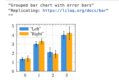
let xs = [0, 1, 2, 3]
let ys1 = [1.35, 3, 2.1, 4]
let ys2 = [1.4, 3.3, 1.9, 4.2]
let yerr1 = [0.2, 0.3, 0.5, 0.4]
let yerr2 = [0.3, 0.3, 0.4, 0.7]

let xs_left = list_map(λ x . x - 0.2, xs)
let xs_right = list_map(λ x . x + 0.2, xs)

diagram(
    bar(xs, ys1, offset = -0.2, width = 0.4, label = "Left"),
    bar(xs, ys2, offset = 0.2, width = 0.4, label = "Right"),
    plot(xs_left, ys1, yerr = yerr1, color = "black", stroke = "none"),
    plot(xs_right, ys2, yerr = yerr2, color = "black", stroke = "none"),
    width = 5,
    legend_position = "left + top"
)
Example: Bar Chart with Dynamic Annotations
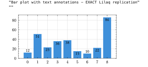
let xs = [0, 1, 2, 3, 4, 5, 6, 7, 8]
let ys = [12, 51, 23, 36, 38, 15, 10, 22, 86]

// Dynamic annotations using list_map and conditionals
let annotations = list_map(λ p .
    let x = fst(p) in
    let y = snd(p) in
    let align = if y > 12 then "top" else "bottom" in
    place(x, y, y, align = align, padding = "0.2em")
, list_zip(xs, ys))

diagram(
    bar(xs, ys),
    annotations,
    width = 9,
    xaxis_subticks = "none"
)
Example: Climograph with Twin Axes
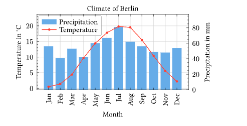
let months = ["Jan", "Feb", "Mar", "Apr", "May", "Jun",
              "Jul", "Aug", "Sep", "Oct", "Nov", "Dec"]
let precipitation = [56, 41, 53, 42, 60, 67, 81, 62, 56, 49, 48, 54]
let temperature = [0.5, 1.4, 4.4, 9.7, 14.4, 17.8, 19.8, 19.5, 15.5, 10.4, 5.6, 2.2]
let xs = range(12)

diagram(
    yaxis(
        bar(xs, precipitation, fill = "blue.lighten(40%)", label = "Precipitation"),
        position = "right",
        axis_label = "Precipitation in mm"
    ),
    plot(xs, temperature, label = "Temperature", color = "red", stroke = "1pt", mark_size = 6),
    width = 8,
    title = "Climate of Berlin",
    ylabel = "Temperature in °C",
    xlabel = "Month",
    xaxis_ticks = months,
    xaxis_tick_rotate = -90,
    xaxis_subticks = "none"
)
Example: Koch Snowflake Fractal
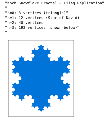
// Complex number operations
define complex_add(c1, c2) = Pair(fst(c1) + fst(c2), snd(c1) + snd(c2))
define complex_sub(c1, c2) = Pair(fst(c1) - fst(c2), snd(c1) - snd(c2))
define complex_mul(c1, c2) = Pair(
    (fst(c1)*fst(c2)) - (snd(c1)*snd(c2)),
    (fst(c1)*snd(c2)) + (snd(c1)*fst(c2))
)

define triangle_vertex(angle) = Pair(cos(radians(angle)), sin(radians(angle)))
define base_triangle() = [triangle_vertex(90), triangle_vertex(210), triangle_vertex(330)]

define koch_edge(p1, p2) =
    let d = complex_sub(p2, p1) in
    [p1, complex_add(p1, complex_mul(d, Pair(1/3, 0))),
     complex_add(p1, complex_mul(d, Pair(0.5, 0 - sqrt(3)/6))),
     complex_add(p1, complex_mul(d, Pair(2/3, 0)))]

define koch_iter(pts) =
    let n = list_length(pts) in
    list_flatten(list_map(λ i .
        koch_edge(list_nth(pts, i), list_nth(pts, mod(i + 1, n)))
    , range(n)))

let n0 = base_triangle()
let n3 = koch_iter(koch_iter(koch_iter(n0)))  // 192 vertices

diagram(
    path(n3, fill = "blue", closed = true),
    width = 6, height = 7,
    xaxis_ticks_none = true,
    yaxis_ticks_none = true
)
Example: Scatter Plot with Colormap
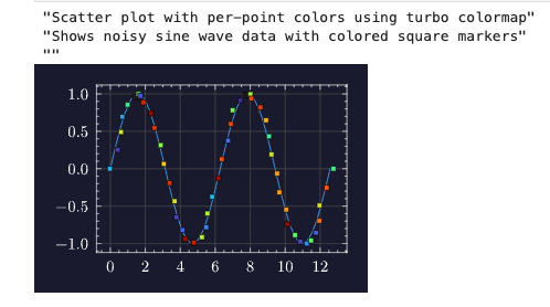
let xs = linspace(0, 12.566370614, 50)  // 0 to 4π
let ys = list_map(lambda x . sin(x), xs)
let noise = random_normal(50, 33, 0.1)
let xs_noisy = vec_add(xs, noise)
let colors = random(50, 42)

diagram(
    plot(xs, ys, mark = "none"),
    scatter(xs_noisy, ys,
        mark = "s",
        colors = colors,
        map = "turbo",
        stroke = "0.5pt + black"
    ),
    theme = "moon"
)
Example: Stacked Area Chart
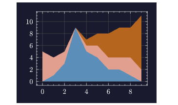
let xs = [0, 1, 2, 3, 4, 5, 6, 7, 8, 9]
let y1 = [0, 1, 3, 9, 5, 4, 2, 2, 1, 0]
let y2 = [5, 3, 2, 0, 1, 2, 2, 2, 3, 2]
let y3 = [0, 0, 0, 0, 1, 2, 4, 5, 5, 9]

diagram(
    stacked_area(xs, y1, y2, y3),
    theme = "moon"
)
Themes
Kleis supports Lilaq’s built-in themes:
| Theme | Description |
|---|---|
schoolbook | Math textbook style with axes at origin |
moon | Dark theme for presentations |
ocean | Blue-tinted theme |
misty | Soft, muted colors |
skyline | Clean, modern look |
diagram(
    plot(xs, ys),
    theme = "moon"
)
Axis Customization
| Option | Description | Example |
|---|---|---|
xlim, ylim | Axis limits | xlim = [-6.28, 6.28] |
xaxis_tick_unit | Tick spacing unit | xaxis_tick_unit = 3.14159 |
xaxis_tick_suffix | Tick label suffix | xaxis_tick_suffix = "pi" |
xaxis_tick_rotate | Rotate labels | xaxis_tick_rotate = -90 |
xaxis_ticks_none | Hide ticks | xaxis_ticks_none = true |
Complete Example Notebook
Cell 1: Import stdlib
import "stdlib/prelude.kleis"
Cell 2: Generate data with linspace
let xs = linspace(0, 6.28, 50)
let ys = list_map(lambda x . sin(x), xs)
Cell 3: Plot with theme
diagram(
    plot(xs, ys, color = "blue", stroke = "2pt"),
    title = "Sine Wave",
    xlabel = "x",
    ylabel = "sin(x)",
    theme = "moon"
)
Logarithmic Scales
For exponential or power-law data, use logarithmic scales:
// Semi-log plot (linear x, logarithmic y)
diagram(
    plot([0, 1, 2, 3, 4], [1, 10, 100, 1000, 10000]),
    title = "Exponential Growth",
    yscale = "log"   // "linear", "log", or "symlog"
)

// Log-log plot (both axes logarithmic)
diagram(
    plot([1, 10, 100, 1000], [1, 100, 10000, 1000000]),
    title = "Power Law",
    xscale = "log",
    yscale = "log"
)
Available scales:
"linear"- Default linear scale"log"- Logarithmic scale (base 10)"symlog"- Symmetric log (linear near 0, log elsewhere; handles negative values)
Next Steps
- Learn to create PDFs, theses, and papers: Document Generation
- Explore the REPL chapter for more interactive features
- See Matrices for symbolic matrix operations
- Check Z3 Verification for formal proofs
Creating Documents with Kleis
Kleis provides a complete document generation system for creating publication-quality theses, dissertations, and papers. Unlike traditional approaches where documents are separate from code, in Kleis your document IS a program.
The Philosophy: Document = Program
Traditional academic writing separates:
- Code (Jupyter notebooks, Python scripts)
- Equations (LaTeX, copy-pasted)
- Plots (matplotlib, exported as images)
- Document (Word, LaTeX, Google Docs)
This separation causes problems:
- Copy-paste errors between code and paper
- Equations that can’t be re-edited
- Plots that can’t be regenerated
- No verification of mathematical claims
Kleis unifies everything into a single program:
┌─────────────────────────────────────────────────────────────┐
│               Your Document (.kleis file)                   │
├─────────────────────────────────────────────────────────────┤
│  Template Import   │ import "stdlib/templates/mit_thesis"   │
│  Metadata          │ Title, author, date, abstract          │
│  Equations         │ MITEquation("label", "$ E = mc^2 $")   │
│  Diagrams          │ MITDiagram("fig1", "caption", code)    │
│  Tables            │ MITTable("tab1", "caption", typst)     │
│  Chapters          │ MITChapter(1, "Introduction", "...")   │
│  Compile Function  │ compile_mit_thesis(my_thesis)          │
└─────────────────────────────────────────────────────────────┘
                              ↓
                   kleis test my_thesis.kleis
                              ↓
                        Typst Output
                              ↓
                   typst compile → PDF
Quick Start
Prerequisites
- Kleis compiled and in PATH
- Typst for PDF generation:
brew install typst
Your First Document (5 minutes)
Create a file my_paper.kleis:
import "stdlib/templates/arxiv_paper.kleis"

// Define your paper
define my_paper = arxiv_paper(
    "My Amazing Research",                    // title
    ["Alice Smith", "Bob Jones"],             // authors
    ["MIT", "Stanford"],                      // affiliations
    "We present groundbreaking results...",   // abstract
    ["machine learning", "verification"],     // keywords
    [
        ArxivSection("Introduction", "We begin by..."),
        ArxivEquation("eq:main", "$ f(x) = x^2 + 1 $"),
        ArxivSection("Methods", "Our approach uses..."),
        ArxivSection("Conclusion", "We have shown...")
    ]
)

// Compile and output
example "compile" {
    let typst = compile_arxiv_paper(my_paper)
    // REQUIRED: typst_raw() makes output unquoted (no "..." around strings)
    // Without it, Typst would see quoted strings and fail to parse
    out(typst_raw(typst))
}
Generate PDF:
# --raw-output suppresses banners (✅/❌), typst_raw() in code produces unquoted output
kleis test --raw-output --example compile my_paper.kleis > my_paper.typ
typst compile my_paper.typ my_paper.pdf
open my_paper.pdf
That’s it! Your document is a Kleis program.
Emit clean Typst (no quotes, no banners)
- Required: Wrap your compiled document in
typst_raw(...)before callingout(...). This is what makes the output unquoted - without it, strings are printed with quotes ("...") which breaks Typst parsing. - Use
table_typst_raw(...)for tables so Typst code is emitted directly (no ASCII boxes). - Run
kleis test --raw-output --example <compile_example> your_doc.kleisto suppress test banners (✅/❌) and summary lines. - Then pipe to
typst compile.
Important: The --raw-output flag only suppresses banners. The typst_raw() wrapper is what produces unquoted output suitable for Typst.
What --raw-output Suppresses
The --raw-output flag suppresses all test framework output:
- Per-example status lines (passed/failed/skipped)
- Error messages after failed examples
- The summary line (“N examples passed” or “N/M examples passed”)
It does not suppress:
- Output from
out()calls in your example blocks (this is what you want to capture) - Exit code 1 on failure (so CI pipelines still detect errors)
Available Templates
Kleis includes three professionally-styled templates:
| Template | File | Use Case |
|---|---|---|
| MIT Thesis | stdlib/templates/mit_thesis.kleis | MIT PhD dissertations |
| UofM Rackham | stdlib/templates/uofm_thesis.kleis | University of Michigan dissertations |
| arXiv Paper | stdlib/templates/arxiv_paper.kleis | arXiv preprints, conference papers |
Each template includes:
- Proper page margins and fonts per institution guidelines
- Title page, abstract, table of contents
- Chapter/section formatting
- Figure, table, and equation support
- Bibliography formatting
- Appendices
Template Gallery
MIT Thesis:
University of Michigan Dissertation:
arXiv Paper:
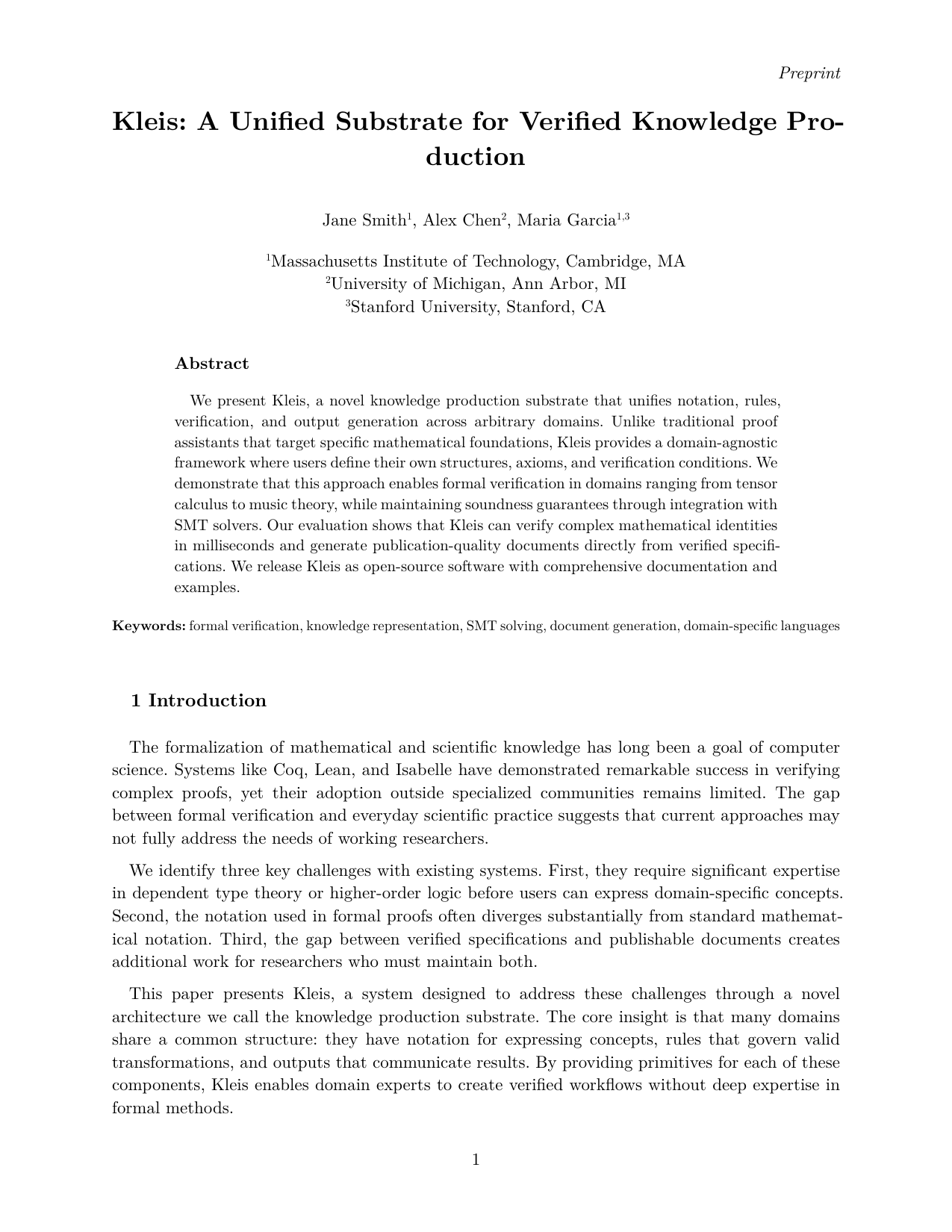
MIT Thesis Template
The MIT thesis template follows the official MIT Libraries thesis specifications.
Document Structure
import "stdlib/templates/mit_thesis.kleis"

// Define thesis metadata
define my_thesis = mit_thesis(
    "Formal Verification of Knowledge Production Systems",  // title
    "Jane Smith",                                            // author
    "Department of EECS",                                    // department
    "May 2026",                                              // date
    PhD,                                                     // degree: SB, SM, or PhD
    "This thesis presents Kleis, a formal verification...", // abstract
    "Prof. Alice Chen",                                      // supervisor
    "Professor of Computer Science",                         // supervisor title
    "I thank my advisor...",                                 // acknowledgments
    "To my family...",                                       // dedication
    all_elements                                             // document content
)
Content Elements
// Chapters
define ch1 = MITChapter(1, "Introduction", "Knowledge production relies on...")

// Sections within chapters
define sec1 = MITSection("Motivation", "The need for formal verification...")

// Subsections
define subsec1 = MITSubsection("Historical Context", "Early work in...")

// Equations
define eq_einstein = MITEquation("eq:einstein", "$ E = m c^2 $")

// Figures (with Typst code)
define fig_arch = MITFigure("fig:arch", "System architecture",
    "#rect(width: 80%, height: 3cm, fill: luma(240))[Architecture diagram]")

// Diagrams using NATIVE KLEIS data
define iterations = [1.0, 2.0, 3.0, 4.0, 5.0]
define accuracy = [10.0, 25.0, 40.0, 55.0, 70.0]
define fig_perf = MITDiagram("fig:perf", "Performance comparison",
    export_typst_fragment(plot(iterations, accuracy, mark = "o"),
        xlabel = "Iterations", ylabel = "Accuracy (%)"))

// Tables using NATIVE KLEIS data
define headers = ["Method", "Accuracy", "Runtime"]
define rows = [["Baseline", "72%", "1.2s"], ["Ours", "89%", "0.8s"]]
define tab_results = MITTable("tab:results", "Experimental results",
    table_typst_raw(headers, rows))

// References
define ref1 = MITReference("demoura2008",
    "de Moura, L. Z3: An Efficient SMT Solver. TACAS 2008.")

// Appendices
define app_a = MITAppendix("Proofs", "Detailed proofs of theorems...")

// Acknowledgments and dedication
define ack = MITAcknowledgments("I thank my advisor...")
define ded = MITDedication("To my family...")
Complete MIT Thesis Example
See the full working example: examples/documents/jane_smith_thesis.kleis
import "stdlib/prelude.kleis"
import "stdlib/templates/mit_thesis.kleis"

// ============================================================================
// JANE SMITH'S PHD THESIS
// ============================================================================

// Chapter 1: Introduction
define ch1 = MITChapter(1, "Introduction",
    "Knowledge production in science relies on precise notation and rigorous
    verification. Traditional approaches separate these concerns...")

// Key equation
define eq_einstein = MITEquation("eq:einstein", "$ E = m c^2 $")

// Performance diagram using NATIVE KLEIS data
define loc = [100.0, 500.0, 1000.0, 5000.0, 10000.0]
define kleis_time = [0.1, 0.3, 0.5, 1.2, 2.1]
define other_time = [0.2, 0.8, 2.0, 12.0, 45.0]

define fig_performance = MITDiagram("fig:perf", "Type inference performance",
    export_typst_fragment(plot(loc, kleis_time, mark = "o", label = "Kleis"),
        xlabel = "Lines of Code", ylabel = "Time (seconds)"))

// Results table using NATIVE KLEIS data
define feature_headers = ["Feature", "Kleis", "Lean", "Coq"]
define feature_rows = [
    ["SMT Integration", "✓", "Partial", "✗"],
    ["Type Inference", "✓", "✓", "✓"],
    ["Typst Export", "✓", "✗", "✗"]
]
define table_features = MITTable("tab:features", "Feature comparison",
    table_typst_raw(feature_headers, feature_rows))

// Assemble all elements in order
define all_elements = [
    ack,           // Acknowledgments (front matter)
    ded,           // Dedication (front matter)
    ch1,           // Chapter 1
    eq_einstein,
    fig_performance,
    ch2,           // Chapter 2
    table_features,
    ch3,           // Chapter 3
    ref1, ref2,    // References
    app_a          // Appendix
]

// Create the thesis
define my_thesis = mit_thesis_full(
    "Formal Verification of Knowledge Production Systems",
    "Jane Smith",
    "Department of Electrical Engineering and Computer Science",
    "May 2026",
    PhD,
    "This thesis presents Kleis, a formal verification system...",
    "Prof. Alice Chen",
    "Professor of Computer Science",
    "I thank my advisor Prof. Chen for her guidance...",
    "To my parents, who taught me to question everything.",
    all_elements
)

// Compile to Typst
example "compile_thesis" {
    let typst = compile_mit_thesis(my_thesis)
    // Emit raw Typst so there are no quotes/escapes
    out(typst_raw(typst))
}
Running the example without banners/quotes: use the raw output mode so the Typst
stream is clean and can be piped directly to typst compile:
./target/release/kleis test examples/documents/jane_smith_thesis.kleis > /tmp/mit_thesis.typ
typst compile /tmp/mit_thesis.typ /tmp/mit_thesis.pdf
What the MIT Template Produces
The compiled thesis includes:
- Title Page - Centered title, author, department, degree, date
- Signature Page - For PhD: supervisor signature block
- Abstract - Formatted per MIT specifications
- Acknowledgments - Optional dedication to advisors, family
- Dedication - Optional short dedication
- Table of Contents - Auto-generated from chapters
- List of Figures - Auto-generated from figures
- List of Tables - Auto-generated from tables
- Chapters - Numbered chapters with sections
- References - Bibliography section
- Appendices - Lettered appendices (A, B, C…)
Table of Contents (auto-generated):
Chapter Content with Equations and Diagrams:
University of Michigan Rackham Template
The UofM template follows Rackham Graduate School formatting guidelines.
Document Structure
import "stdlib/templates/uofm_thesis.kleis"

// Committee members
define committee = [
    committee_member("Prof. Alice Chen", "Computer Science"),
    committee_member("Prof. Bob Smith", "Mathematics"),
    committee_member("Prof. Carol Davis", "Statistics")
]

// Define dissertation
define my_dissertation = umich_dissertation(
    "Deep Learning Theory and Applications",      // title
    "Alex Chen",                                  // author
    "Computer Science and Engineering",           // program
    "2026",                                       // year
    PhD,                                          // degree
    "This dissertation investigates...",          // abstract
    "Prof. Alice Chen",                           // committee chair
    "Computer Science and Engineering",           // chair affiliation
    committee,                                    // committee list
    "achen@umich.edu",                           // email
    "0000-0001-2345-6789",                       // ORCID
    "I thank the Rackham Graduate School...",    // acknowledgments
    "To my mentors...",                          // dedication
    "This work began as...",                     // preface
    all_elements                                 // content
)
UofM-Specific Features
- Double spacing throughout (Rackham requirement)
- Identifier page with ORCID and email
- Committee page with full committee list
- Preface section (optional)
- 2-inch top margin on chapter openings
- Roman numerals for front matter pages
Complete UofM Example
See: examples/documents/alex_chen_dissertation.kleis
Run the provided compile block with raw output to get Typst ready for typst compile:
./target/release/kleis test examples/documents/alex_chen_dissertation.kleis > /tmp/umich.typ
typst compile /tmp/umich.typ /tmp/umich.pdf
arXiv Paper Template
The arXiv template follows common academic paper conventions for preprints.
Document Structure
import "stdlib/templates/arxiv_paper.kleis"

define my_paper = arxiv_paper_full(
    "Attention Is All You Need",                          // title
    ["Ashish Vaswani", "Noam Shazeer", "Niki Parmar"],   // authors
    ["Google Brain", "Google Brain", "Google Research"], // affiliations
    "The dominant sequence transduction models...",       // abstract
    ["transformers", "attention", "neural networks"],    // keywords
    all_elements                                          // content
)
arXiv Content Elements
// Sections (no chapters in papers)
ArxivSection("Introduction", "Recent advances in...")
ArxivSection("Related Work", "Prior work includes...")

// Equations
ArxivEquation("eq:attention", "$ \\text{Attention}(Q, K, V) = \\text{softmax}(QK^T / \\sqrt{d_k})V $")

// Algorithms (using Typst's algo package)
ArxivAlgorithm("alg:train", "Training procedure", "
#import \"@preview/algorithmic:0.1.0\"
#algorithmic.algorithm({
  algorithmic.For(cond: [epoch in 1..N])[
    algorithmic.For(cond: [batch in data])[
      Compute loss and update
    ]
  ]
})
")

// Figures, tables, diagrams (same as MIT)
ArxivFigure("fig:model", "Model architecture", "...")
define result_headers = ["Method", "Accuracy", "Runtime"]
define result_rows = [["Baseline", "72%", "1.2s"], ["Ours", "89%", "0.8s"]]
ArxivTable("tab:results", "Experimental results",
    table_typst_raw(result_headers, result_rows))
ArxivDiagram("fig:loss", "Training loss", "...")

// Acknowledgments
ArxivAcknowledgments("We thank the Google Brain team...")

// References
ArxivReference("vaswani2017", "Vaswani et al. Attention Is All You Need. NeurIPS 2017.")

// Appendices
ArxivAppendix("Implementation Details", "We used PyTorch...")
Complete arXiv Example
See: examples/documents/sample_arxiv_paper.kleis
Diagrams and Plots
Kleis integrates with the Lilaq plotting library for creating beautiful diagrams directly in your document.
Native Kleis Data (Recommended)
The most powerful approach uses native Kleis lists with export_typst_fragment():
// Define your data as Kleis lists
define epochs = [1.0, 2.0, 3.0, 4.0, 5.0]
define accuracy = [10.0, 25.0, 45.0, 70.0, 90.0]

// Create a plot using Kleis's native plot() function
define my_plot = plot(epochs, accuracy, mark = "o", label = "Training")

// Convert to Typst code for embedding in a figure
define typst_code = export_typst_fragment(my_plot,
    title = "Model Performance",
    xlabel = "Epoch",
    ylabel = "Accuracy (%)"
)

// Use in your thesis/paper
define fig_training = MITDiagram("fig:training", "Training curves", typst_code)
Note: When piping to typst:
- Use
--raw-outputto suppress test banners (✅/❌) - Use
--example compileto run only the compile example - Ensure your example uses
out(typst_raw(...))for unquoted output
./target/release/kleis test --raw-output --example compile examples/documents/sample_arxiv_paper.kleis > /tmp/paper.typ
typst compile /tmp/paper.typ /tmp/paper.pdf
Why use native data?
- Your data is Kleis—it can be computed, verified, and reused
- No manual Typst syntax errors
- Data can flow from experiments to figures seamlessly
- Easier to update when results change
Available Plot Functions
| Function | Description |
|---|---|
plot(xs, ys) | Line plot |
scatter(xs, ys) | Scatter plot |
bar(xs, heights) | Vertical bar chart |
hbar(xs, widths) | Horizontal bar chart |
Each function accepts optional parameters: label, mark, stroke, etc.
Example: Complete Workflow
// Raw experimental data
define x_data = [0.1, 0.5, 1.0, 5.0, 10.0, 25.0]
define method_a = [150.0, 120.0, 100.0, 80.0, 60.0, 40.0]
define method_b = [180.0, 140.0, 110.0, 85.0, 65.0, 45.0]
// Create plots
define plot_a = plot(x_data, method_a, mark = "o", label = "Method A")
define plot_b = plot(x_data, method_b, mark = "x", label = "Method B")
// Combine into diagram
define comparison_typst = export_typst_fragment(plot_a,
title = "Performance Comparison",
xlabel = "Problem Size",
ylabel = "Time (ms)"
)
// Embed in thesis
define fig_comparison = MITDiagram("fig:comparison",
"Performance comparison between methods",
comparison_typst
)
Fallback: Raw Typst Strings
For complex diagrams not yet supported by native functions, you can use raw Typst strings:
define fig_complex = MITDiagram("fig:complex", "Complex diagram", "
import \"@preview/lilaq:0.5.0\" as lq
lq.diagram(
lq.plot((1, 2, 3, 4), (10, 20, 35, 50), stroke: blue, mark: \"o\"),
lq.plot((1, 2, 3, 4), (15, 30, 42, 55), stroke: red, mark: \"x\"),
xlabel: \"Iteration\",
ylabel: \"Value\"
)")
Tables
Native Kleis Data with table_typst_raw() (Recommended)
The cleanest approach uses Kleis lists with table_typst_raw(), which emits Typst directly (no quotes, no ASCII boxes):
// Define table data as Kleis lists
define headers = ["Method", "Accuracy", "F1 Score"]
define rows = [
["Baseline", "72.3%", "0.71"],
["Ours", "89.7%", "0.88"],
["SOTA", "87.1%", "0.86"]
]
// Generate Typst table code (raw Typst)
define table_code = table_typst_raw(headers, rows)
// Use in your thesis/paper
define tab_results = MITTable("tab:results", "Benchmark results", table_code)
Why use table_typst_raw()?
- Data as Kleis lists—can be computed, imported, or transformed
- No manual Typst table syntax
- Rows can come from experiments or external data
- Easy to add/remove rows programmatically
- Produces clean Typst for piping to
typst compile
Example: Complete Workflow
// Data from experiments
define methods = ["CNN", "ResNet", "Transformer", "Kleis-Net"]
define accuracy = ["72.3%", "85.1%", "87.4%", "89.7%"]
define f1_scores = ["0.71", "0.84", "0.86", "0.88"]
define memory = ["128 MB", "256 MB", "512 MB", "192 MB"]
// Build table from data
define headers = ["Method", "Accuracy", "F1", "Memory"]
define rows = [
["CNN", "72.3%", "0.71", "128 MB"],
["ResNet", "85.1%", "0.84", "256 MB"],
["Transformer", "87.4%", "0.86", "512 MB"],
["Kleis-Net", "89.7%", "0.88", "192 MB"]
]
define tab_comparison = MITTable("tab:comparison",
"Comparison of deep learning methods",
table_typst_raw(headers, rows)
)
Fallback: Raw Typst Strings
For styled tables, you can use raw Typst syntax:
define tab_styled = MITTable("tab:styled", "Styled table", "
#table(
columns: 4,
stroke: 0.5pt,
fill: (col, row) => if row == 0 { luma(230) },
[Feature], [Kleis], [Lean], [Coq],
[SMT], [✓], [Partial], [✗],
[Types], [HM], [Dependent], [Dependent]
)")
Equations
Equations use Typst math syntax (similar to LaTeX):
// Simple equation
MITEquation("eq:simple", "$ x = \\frac{-b \\pm \\sqrt{b^2 - 4ac}}{2a} $")
// Multi-line equation
MITEquation("eq:multi", "$
\\nabla \\cdot E &= \\frac{\\rho}{\\epsilon_0} \\
\\nabla \\cdot B &= 0 \\
\\nabla \\times E &= -\\frac{\\partial B}{\\partial t} \\
\\nabla \\times B &= \\mu_0 J + \\mu_0 \\epsilon_0 \\frac{\\partial E}{\\partial t}
$")
// Inline math in text - just use $...$
MITSection("Methods", "A function $f: RR^n -> RR^m$ maps inputs to outputs.")
// Literal dollar sign - use \$
MITSection("Cost", "The price is \\$100 per unit.")
Common Math Symbols
| Symbol | Typst | Example |
|---|---|---|
| Fraction | frac(a, b) | $ \frac{a}{b} $ |
| Square root | sqrt(x) | $ \sqrt{x} $ |
| Summation | sum_(i=0)^n | $ \sum_{i=0}^n $ |
| Integral | integral_a^b | $ \int_a^b $ |
| Greek | alpha, beta, gamma | α, β, γ |
| Subscript | x_i | $ x_i $ |
| Superscript | x^2 | $ x^2 $ |
| Partial | partial | ∂ |
| Nabla | nabla | ∇ |
💡 Tip: Use the Equation Editor
You don’t have to type Typst syntax manually!
The Kleis Equation Editor is a visual, WYSIWYG tool for building equations. Instead of memorizing frac(a, b) or mat(delim: "[", ...), you:
- Build visually — Click buttons to create fractions, matrices, integrals
- See live preview — The equation renders as you build (powered by Typst)
- Copy and paste — Click “📋 Copy Typst” and paste into your thesis
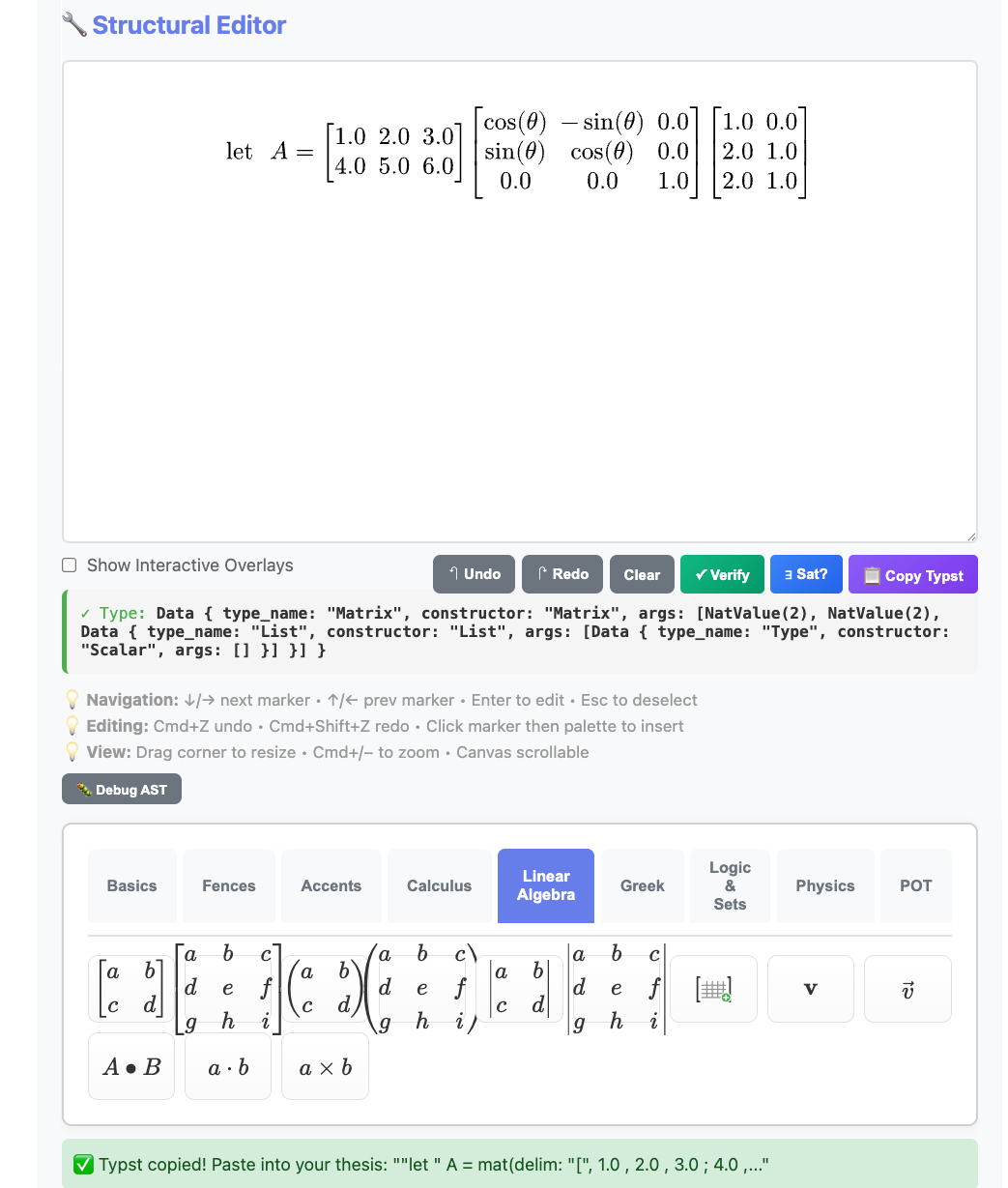
The Equation Editor showing a type-checked matrix multiplication with rotation matrix. The type indicator confirms: Matrix(2, 2, Scalar).
The workflow:
Visual Editor → 📋 Copy Typst → Paste into thesis.kleis → PDF
Example: Building let A = [1 2 3; 4 5 6] × R_z(θ) × [1 0; 2 1; 2 1] takes seconds visually — versus minutes of typing and debugging Typst syntax.
Note: The Equation Editor requires
kleis serverrunning:kleis server # Server running at http://localhost:3000Then open http://localhost:3000 in your browser. Full documentation coming in a future chapter.
Generating PDFs
Command Line
# Compile Kleis to Typst
# --raw-output: suppresses ✅/❌ banners
# --example compile: runs only the "compile" example block
# Your example must use out(typst_raw(...)) for unquoted output
kleis test --raw-output --example compile my_thesis.kleis > my_thesis.typ
# Compile Typst to PDF
typst compile my_thesis.typ my_thesis.pdf
# Open PDF (macOS)
open my_thesis.pdf
One-liner
kleis test --raw-output --example compile my_thesis.kleis > my_thesis.typ && typst compile my_thesis.typ && open my_thesis.pdf
From Jupyter
Jupyter is the recommended environment for writing your thesis. Here’s a complete workflow:
Cell 1: Setup and check templates
from kleis_kernel import compile_to_pdf, compile_to_typst, list_templates, validate
# See available templates
print("Available templates:", list_templates())
# Output: ['mit_thesis', 'uofm_thesis', 'arxiv_paper']
Cell 2: Validate your document
# Check for parse errors before compiling
validate("my_thesis.kleis")
# Output: ✓ my_thesis.kleis is valid
Cell 3: Generate PDF
# Compile Kleis → Typst → PDF
compile_to_pdf("my_thesis.kleis", "my_thesis.pdf")
# Output: ✓ PDF created: my_thesis.pdf
Cell 4: Display in notebook
from IPython.display import IFrame
IFrame("my_thesis.pdf", width=800, height=600)
Alternative: View Typst output
# See the generated Typst code (useful for debugging)
typst_code = compile_to_typst("my_thesis.kleis")
print(typst_code[:500]) # First 500 chars
Complete Jupyter Workflow Example
# ============================================================
# Thesis Writing Workflow in Jupyter
# ============================================================
from kleis_kernel import compile_to_pdf, validate
from IPython.display import IFrame
import os
# 1. Your thesis file (edit this in VS Code or any text editor)
THESIS_FILE = "my_thesis.kleis"
# 2. Validate before compiling
if validate(THESIS_FILE):
# 3. Generate PDF
compile_to_pdf(THESIS_FILE, "thesis_draft.pdf")
# 4. Display inline
display(IFrame("thesis_draft.pdf", width=800, height=600))
else:
print("Fix the errors above, then re-run this cell")
Tips for Jupyter Users
- Edit
.kleisfiles externally - Use VS Code with syntax highlighting - Use Jupyter for compilation - Quick feedback loop
- Version control - Git works great with
.kleisfiles (they’re plain text) - Hot reload - Re-run the cell after editing your
.kleisfile
Creating Custom Templates
To create a new template (e.g., for IEEE or Nature), create a .kleis file:
// stdlib/templates/ieee_paper.kleis
import "stdlib/prelude.kleis"
// Template metadata
define template_name = "IEEE Paper"
define template_version = "1.0"
define template_type = "paper"
// Data types for document elements
data IEEEDocExpr =
IEEESection(title: String, content: String)
| IEEEEquation(label: String, typst_code: String)
| IEEEFigure(label: String, caption: String, typst_code: String)
| IEEETable(label: String, caption: String, typst_code: String)
| IEEEReference(key: String, citation: String)
// Document container
data IEEEPaper = IEEEPaper(
title: String,
authors: List(String),
affiliations: List(String),
abstract_text: String,
keywords: List(String),
elements: List(IEEEDocExpr)
)
// Typst styling
define typst_ieee_page_setup = "#set page(
paper: \"us-letter\",
margin: (top: 0.75in, bottom: 1in, left: 0.625in, right: 0.625in),
columns: 2
)"
define typst_ieee_text_setup = "#set text(
font: \"Times New Roman\",
size: 10pt
)"
// ... more styling definitions ...
// Compile function
define compile_ieee_paper(paper) =
match paper {
IEEEPaper(title, authors, affiliations, abstract_text, keywords, elements) =>
concat(typst_ieee_page_setup,
concat(typst_ieee_text_setup,
// ... assemble document ...
))
}
No Rust code changes needed! Just add the template file.
Tips for Thesis Writing
- Save frequently — Your
.kleisfile is the source of truth - Use version control —
.kleisfiles are text, perfect for git - Label everything — Use meaningful labels for cross-references
- Test incrementally — Compile often to catch errors early
- Use Lilaq for plots — Regenerable, not static images
- Store in one file — Keep related content together
Troubleshooting
“Typst not found”
# macOS
brew install typst
# Linux
curl -fsSL https://typst.app/install.sh | sh
“Parse error in .kleis file”
Check for:
- Unescaped quotes in strings (use
\") - Missing commas in lists
- Unclosed parentheses
“Figure not rendering”
Ensure Lilaq import is correct in your diagram code:
import "@preview/lilaq:0.5.0" as lq
“Cross-reference not found”
Labels must match exactly:
MITEquation("eq:main", "...") // Define
"See Equation @eq:main" // Reference
Next Steps
- See how documents combine with verification: Applications
- See full examples in
examples/documents/ - Explore Typst documentation: typst.app/docs
- Learn Lilaq plotting: Lilaq on Typst Universe
Applications
Kleis is designed for mathematical verification, but its power extends far beyond pure mathematics. This chapter showcases applications across multiple domains.
Note: Many examples in this chapter use
exampleblocks withassertstatements for testing and verification. See Example Blocks for details on this syntax.
AI/ML Verification
Kleis aligns with the research agenda outlined in “Toward Verified Artificial Intelligence” (Seshia et al., Communications of the ACM, 2022) — a seminal paper from UC Berkeley on using formal methods to verify AI systems.
The Verified AI Challenge
The paper identifies five key challenges for AI verification:
| Challenge | Description | Kleis Approach |
|---|---|---|
| Environment Modeling | Formally specify the world | structure with axioms |
| Specification | Define “correct” behavior | First-order logic assertions |
| Computational Engines | SAT/SMT solving | Z3 backend |
| Correct-by-Construction | Build verified from start | Axiom-first development |
| Compositional Reasoning | Modular proofs | implements contracts |
Neural Network Properties
Kleis can express and verify properties of neural networks:
// Robustness: Small input changes → small output changes
structure RobustnessProperty {
axiom local_robustness: ∀ x : Input . ∀ δ : Input .
norm(δ) < ε →
abs(network(x + δ) - network(x)) < bound
}
// Monotonicity: Larger input → larger output (for certain features)
structure MonotonicityProperty {
axiom monotonic_feature: ∀ x1 : Input . ∀ x2 : Input .
x1.feature ≤ x2.feature →
network(x1) ≤ network(x2)
}
// Safety envelope: Output always in safe region
structure SafetyProperty {
axiom output_bounded: ∀ x : Input .
valid_input(x) →
min_safe ≤ network(x) ∧ network(x) ≤ max_safe
}
Safe Reinforcement Learning
// Safety envelope for learning-based controllers
structure SafeController(state_dim: Nat, action_dim: Nat) {
// Pre-computed safety region
element safe_set : Set(State)
// Learned policy
operation policy : State → Action
// Safety invariant: policy never leaves safe set
axiom safety_invariant: ∀ s : State .
s ∈ safe_set →
next_state(s, policy(s)) ∈ safe_set
// Backup controller for edge cases
operation backup : State → Action
axiom backup_safe: ∀ s : State .
next_state(s, backup(s)) ∈ safe_set
}
Compositional Verification
The paper emphasizes assume-guarantee reasoning — exactly what Kleis structures provide:
// Perception module contract
structure PerceptionContract {
operation detect : Image → List(BoundingBox)
// Guarantee: no false negatives within sensor range
axiom no_miss_close: ∀ img : Image . ∀ obj : Object .
distance(obj) < sensor_range ∧ visible(obj, img) →
∃ box : BoundingBox . box ∈ detect(img) ∧ contains(box, obj)
}
// Planning module contract
structure PlanningContract {
// Assume: perception is correct within range
// Guarantee: plan avoids all detected obstacles
axiom collision_free: ∀ boxes : List(BoundingBox) . ∀ plan : Trajectory .
plan = plan_path(boxes) →
∀ t : Time . ∀ box : BoundingBox .
box ∈ boxes → ¬intersects(plan(t), box)
}
// System-level property emerges from composition
structure SystemSafety {
axiom no_collision: ∀ img : Image .
let boxes = PerceptionContract.detect(img) in
let plan = PlanningContract.plan_path(boxes) in
collision_free(plan)
}
Why Kleis for AI Verification?
| Approach | Limitation | Kleis Advantage |
|---|---|---|
| Testing | Samples finite cases | Proves ∀ inputs |
| Fuzzing | Random, no guarantees | Exhaustive (for decidable) |
| Static analysis | Over-approximates | Precise via Z3 |
| Runtime monitoring | Reactive only | Proactive verification |
Further Reading
- Paper: Toward Verified Artificial Intelligence (CACM 2022)
- VerifAI: Toolkit for formal AI verification (same authors)
- Scenic: Domain-specific language for scenario specification
Kleis provides a general-purpose substrate for expressing the same verification concepts in a unified, mathematically rigorous framework.
Hardware Verification
Kleis can formally verify hardware designs using Z3’s bitvector theory. This section explains how Kleis compares to the industry-standard Universal Verification Methodology (UVM) defined in IEEE 1800.2-2020.
Kleis vs UVM: Different Approaches to the Same Goal
| Aspect | UVM (IEEE 1800.2) | Kleis |
|---|---|---|
| Verification method | Simulation (random sampling) | Formal proof (Z3) |
| Coverage | Statistical: “did we test this?” | Exhaustive: “is this state reachable?” |
| Assertions | SVA (temporal, simulation-checked) | First-order logic (mathematically proven) |
| Language | SystemVerilog class library | Native Kleis |
| Cost | Requires commercial simulators | Open source |
What Kleis Proves
Kleis can formally prove properties for ALL possible inputs:
// Bitvector operations (maps to SystemVerilog bit[7:0])
operation bvadd : BitVec8 × BitVec8 → BitVec8
operation bvxor : BitVec8 × BitVec8 → BitVec8
operation bv_zero : BitVec8
// PROVE: Addition is commutative for ALL 2^16 input pairs
example "ADD is commutative" {
assert(∀ a : BitVec8 . ∀ b : BitVec8 . bvadd(a, b) = bvadd(b, a))
}
// PROVE: XOR of same value always yields zero
example "XOR self is zero" {
assert(∀ a : BitVec8 . bvxor(a, a) = bv_zero)
}
// PROVE: Subtraction inverts addition
example "SUB inverts ADD" {
assert(∀ a : BitVec8 . ∀ b : BitVec8 . bvsub(bvadd(a, b), b) = a)
}
A UVM testbench would run random tests and hope to find bugs. Kleis proves correctness mathematically.
Reachability Analysis (Related to Coverage)
UVM coverage answers: “Did our tests exercise this state?”
Kleis reachability answers: “Is this state possible at all?”
// Can ADD ever produce zero? (Yes: 0+0, or 128+128 with overflow)
example "Zero is reachable via ADD" {
assert(∃ a : BitVec8 . ∃ b : BitVec8 . bvadd(a, b) = bv_zero)
}
// Can ADD produce non-zero? (Yes: 1+0, etc.)
example "Non-zero is reachable via ADD" {
assert(∃ a : BitVec8 . ∃ b : BitVec8 . bvadd(a, b) ≠ bv_zero)
}
Kleis Complements UVM, Not Replaces It
Kleis and UVM solve related but different problems:
┌─────────────────────────────────────────────────────────────┐
│ VERIFICATION WORKFLOW │
├─────────────────────────────────────────────────────────────┤
│ │
│ KLEIS (Pre-RTL) UVM (With RTL) │
│ ┌────────────────┐ ┌────────────────┐ │
│ │ Define ALU │ │ Verilog ALU │ │
│ │ specification │ → │ implementation │ │
│ └────────────────┘ └────────────────┘ │
│ ↓ ↓ │
│ ┌────────────────┐ ┌────────────────┐ │
│ │ PROVE correct │ │ SIMULATE with │ │
│ │ for ALL inputs │ │ random tests │ │
│ └────────────────┘ └────────────────┘ │
│ ↓ ↓ │
│ Mathematical "Probably correct" │
│ certainty (statistical) │
│ │
└─────────────────────────────────────────────────────────────┘
Use Kleis FIRST: Prove your algorithm is correct before writing HDL.
Use UVM AFTER: Validate your Verilog/VHDL implements the algorithm correctly.
What UVM Has That Kleis Doesn’t
| UVM Feature | Kleis Status | Notes |
|---|---|---|
| DUT connection | Not applicable | Kleis doesn’t connect to HDL |
| Timing/clocks | Different paradigm | Model time explicitly if needed |
| Sequences over time | Not needed | Kleis proves for all states |
| Transaction-level modeling | Can model | Use data types |
| Waveform output | Not applicable | No simulation |
Example: ALU Verification
See examples/hardware/alu_verification.kleis for a complete example that proves:
- ADD/AND/OR/XOR commutativity
- Addition associativity
- Subtraction inverts addition
- AND idempotence
- XOR self produces zero
- Additive inverse
- Reachability of zero and non-zero results
All properties are proven for all 65,536 possible 8-bit input pairs — not sampled, but exhaustively verified.
When to Use Kleis for Hardware
| Use Case | Kleis? | Why |
|---|---|---|
| Algorithm correctness before RTL | Yes | Prove before you code |
| Property verification | Yes | Mathematical proof |
| Bug hunting in existing RTL | No | Use UVM/formal tools |
| Coverage closure | Partial | Reachability, not statistical |
| Integration with HDL flow | No | Standalone verification |
Business Process Modeling
Model and verify business workflows with formal guarantees:
// Order-to-Cash (O2C) Business Process
// Models the complete lifecycle from order to payment
// Order lifecycle states
data OrderStatus =
Draft | Pending | CreditApproved | CreditDenied
| Allocated | Fulfilled | Shipped | Invoiced
| Paid | Complete | Cancelled
// Credit check decision based on utilization
define credit_check_decision(utilization) =
if utilization <= 100 then 1 // Approved
else if utilization < 125 then 2 // PendingReview
else 0 // Denied
// Can order be cancelled from current state?
define can_cancel(status) = match status {
Draft => 1
| Pending => 1
| CreditApproved => 1
| Allocated => 1
| _ => 0 // Can't cancel after fulfillment
}
// INVARIANT: No shipment without credit approval
define shipment_requires_credit(order_status, credit_approved) =
if order_status = 6 then credit_approved = 1 else true
// INVARIANT: Order completion requires full payment
define completion_requires_payment(order_status, payment_status) =
if order_status = 9 then payment_status >= 2 else true
Network Protocol Verification
Verify protocol correctness with formal methods:
// Stop-and-Wait Protocol - Reliable Data Transfer
// Sequence numbers alternate between 0 and 1
define next_seq(seq) = if seq = 0 then 1 else 0
// ACK is valid if it matches sent sequence
define valid_ack(sent, ack) = if ack = sent then 1 else 0
// Sender advances state only on valid ACK
define sender_next_state(current_seq, ack_received) =
if valid_ack(current_seq, ack_received) = 1
then next_seq(current_seq)
else current_seq
// VERIFIED: Double alternation returns to original
// next_seq(next_seq(0)) = 0 ✓
// next_seq(next_seq(1)) = 1 ✓
// SAFETY: No duplicate delivery when synchronized
// LIVENESS: Progress guaranteed when channel delivers
IPv4 Packet Validation
// IPv4 Header Validation (RFC 791)
// Version must be 4 for IPv4
define valid_version(v) = if v = 4 then 1 else 0
// IHL (Internet Header Length): 5-15 words
define valid_ihl(ihl) = ihl >= 5 and ihl <= 15
// Header length in bytes
define header_length(ihl) = ihl * 4
// Common protocols: 1=ICMP, 6=TCP, 17=UDP
define is_tcp(proto) = proto = 6
define is_udp(proto) = proto = 17
// Private address ranges
define is_private_class_a(o1) = o1 = 10
define is_private_class_c(o1, o2) = o1 = 192 and o2 = 168
// Full packet validation
define valid_packet(version, ihl, total, ttl, proto) =
valid_version(version) = 1 and
valid_ihl(ihl) = 1 and
ttl > 0 and
total >= header_length(ihl)
Authorization & Access Control
Model Zanzibar-style relationship-based access control (like Google Drive):
// Permission Levels: 0=None, 1=Viewer, 2=Commenter, 3=Editor, 4=Owner
define has_at_least(user_perm, required_perm) = user_perm >= required_perm
define can_read(perm) = has_at_least(perm, 1)
define can_edit(perm) = has_at_least(perm, 3)
define can_delete(perm) = has_at_least(perm, 4)
// Folder inheritance (like Google Drive)
define inherited_permission(child_perm, parent_perm) =
if child_perm > 0
then child_perm // Explicit permission overrides
else parent_perm // Inherit from parent
// Multi-group permission: take highest
define effective_permission(direct, group) =
if direct >= group then direct else group
// Security invariant: can_edit implies can_read
// ∀ p . can_edit(p) = 1 → can_read(p) = 1
Security Analysis
Use Z3 string theory for static security analysis:
// SQL Injection Detection using String Operations
// Vulnerable pattern: string concatenation + SQL execution
// :verify and(
// contains("SELECT * FROM users WHERE id=" + userId, "+ userId"),
// contains(code, "executeQuery")
// )
// If Valid → VULNERABLE!
// Safe pattern: parameterized queries
// :verify and(
// contains(code, "PreparedStatement"),
// not(contains(code, "+ userId +"))
// )
// If Valid → SAFE
// XSS Detection: innerHTML with user input
// :verify and(
// contains(code, "innerHTML"),
// contains(code, "userData")
// )
Control Systems Engineering
Design optimal controllers with verified stability:
// LQG Controller: Linear Quadratic Gaussian
structure LinearSystem(n: Nat, m: Nat, p: Nat) {
element A : Matrix(n, n, ℝ) // State dynamics
element B : Matrix(n, m, ℝ) // Input matrix
element C : Matrix(p, n, ℝ) // Output matrix
element W : Matrix(n, n, ℝ) // Process noise covariance
element V : Matrix(p, p, ℝ) // Measurement noise covariance
}
// LQR: Optimal state feedback
operation lqr_gain : LQRProblem(n, m) → Matrix(m, n, ℝ)
axiom lqr_stability:
∀ prob : LQRProblem(n, m) .
let K = lqr_gain(prob) in
let A_cl = prob.A - prob.B · K in
is_stable(A_cl)
// Kalman Filter: Optimal state estimation
operation kalman_gain : KalmanProblem(n, p) → Matrix(n, p, ℝ)
// LQG combines LQR + Kalman via Separation Principle
structure LQGController(n: Nat, m: Nat, p: Nat) {
element K : Matrix(m, n, ℝ) // LQR gain
element L : Matrix(n, p, ℝ) // Kalman gain
}
Dimensional Analysis (Physical Units)
Prevent unit mismatch bugs at compile time - like the Mars Climate Orbiter disaster ($327M lost due to imperial/metric confusion):
// Physical dimensions as exponent tuples [Length, Mass, Time]
structure Dimension(L : ℤ, M : ℤ, T : ℤ) {
axiom equal : ∀(d1 d2 : Dimension).
d1 = d2 ↔ (L(d1) = L(d2) ∧ M(d1) = M(d2) ∧ T(d1) = T(d2))
}
// Named dimensions
define Length = Dimension(1, 0, 0)
define Mass = Dimension(0, 1, 0)
define Time = Dimension(0, 0, 1)
define Velocity = Dimension(1, 0, -1) // L·T⁻¹
define Force = Dimension(1, 1, -2) // M·L·T⁻²
define Energy = Dimension(2, 1, -2) // M·L²·T⁻²
// Physical quantity = value + dimension
structure Quantity(value : ℝ, dim : Dimension) {
// Addition: dimensions must match
axiom add_same_dim : ∀(q1 q2 : Quantity)(d : Dimension).
dim(q1) = d ∧ dim(q2) = d → dim(q1 + q2) = d
// Multiplication: dimensions compose
axiom mul_composes : ∀(q1 q2 : Quantity).
dim(q1 * q2) = Dimension(
L(dim(q1)) + L(dim(q2)),
M(dim(q1)) + M(dim(q2)),
T(dim(q1)) + T(dim(q2)))
}
// Unit constructors
define meter(x : ℝ) = Quantity(x, Length)
define kilogram(x : ℝ) = Quantity(x, Mass)
define second(x : ℝ) = Quantity(x, Time)
define newton(x : ℝ) = Quantity(x, Force)
// Physics axioms verify dimensional consistency
structure Mechanics {
// F = ma: [M·L·T⁻²] = [M] × [L·T⁻²] ✓
axiom newton_second_law : ∀(m : Quantity)(a : Quantity).
dim(m) = Mass ∧ dim(a) = Dimension(1, 0, -2) →
dim(m * a) = Force
// E = ½mv²: [M·L²·T⁻²] = [M] × [L·T⁻¹]² ✓
axiom kinetic_energy : ∀(m : Quantity)(v : Quantity).
dim(m) = Mass ∧ dim(v) = Velocity →
dim(m * v * v) = Energy
}
Type-safe physics:
meter(100) + meter(50)→Quantity(150, Length)✓meter(100) / second(10)→Quantity(10, Velocity)✓meter(100) + second(10)→ ❌ Type error:Length ≠ Time
See examples/physics/dimensional_analysis.kleis for the full example.
Differential Geometry
Kleis excels at differential geometry calculations:
// Christoffel symbols for spherical coordinates
structure SphericalMetric {
operation metric : (ℝ, ℝ) → Matrix(2, 2, ℝ)
operation christoffel : (ℝ, ℝ) → Tensor(1, 2)
}
implements SphericalMetric {
// Metric tensor: ds² = r²(dθ² + sin²θ dφ²)
operation metric(r, θ) = Matrix [
[r^2, 0],
[0, r^2 * sin(θ)^2]
]
// Christoffel symbols Γⁱⱼₖ
operation christoffel(r, θ) =
let g = metric(r, θ) in
let g_inv = inverse(g) in
// ... compute from metric derivatives
}
Tensor Calculus
// Einstein field equations
structure EinsteinEquations {
// Ricci tensor
operation ricci : Manifold → Tensor(0, 2)
// Scalar curvature
operation scalar : Manifold → ℝ
// Einstein tensor
operation einstein : Manifold → Tensor(0, 2)
axiom einstein_tensor : ∀(M : Manifold).
einstein(M) = ricci(M) - (scalar(M) / 2) * metric(M)
}
Symbolic Differentiation
Kleis supports differentiation in two fundamentally different ways:
| Approach | Function | Purpose | Runs In |
|---|---|---|---|
| Computational | diff(expr, var) | Actually compute derivatives | Kleis Evaluator |
| Axiomatic | D(f, x), Dt(f, x) | Verify derivative properties | Z3 Solver |
Computational Differentiation: diff
The diff function computes derivatives by pattern matching on expression trees. It’s implemented in pure Kleis and returns a new expression:
data Expression =
ENumber(value : ℝ)
| EVariable(name : String)
| EOperation(name : String, args : List(Expression))
// Helper constructors
define num(n) = ENumber(n)
define var(x) = EVariable(x)
define e_add(a, b) = EOperation("plus", Cons(a, Cons(b, Nil)))
define e_mul(a, b) = EOperation("times", Cons(a, Cons(b, Nil)))
define e_pow(a, b) = EOperation("power", Cons(a, Cons(b, Nil)))
define diff(e, var_name) =
match e {
ENumber(_) => num(0)
EVariable(name) => if str_eq(name, var_name) then num(1) else num(0)
EOperation(op_name, args) => diff_op(op_name, args, var_name)
}
define diff_op(op_name, args, var_name) = match op_name {
"plus" => match args {
Cons(f, Cons(g, Nil)) => e_add(diff(f, var_name), diff(g, var_name))
| _ => num(0)
}
"times" => match args {
Cons(f, Cons(g, Nil)) =>
e_add(e_mul(diff(f, var_name), g), e_mul(f, diff(g, var_name)))
| _ => num(0)
}
"power" => match args {
Cons(f, Cons(ENumber(n), Nil)) =>
e_mul(e_mul(num(n), e_pow(f, num(n - 1))), diff(f, var_name))
| _ => num(0)
}
"sin" => match args {
Cons(f, Nil) => e_mul(e_cos(f), diff(f, var_name))
| _ => num(0)
}
"cos" => match args {
Cons(f, Nil) => e_neg(e_mul(e_sin(f), diff(f, var_name)))
| _ => num(0)
}
_ => num(0)
}
Usage: Call diff(e_mul(var("x"), var("x")), "x") and get back an expression representing 2x.
Axiomatic Differentiation: D and Dt
The D and Dt operations are declared in stdlib/calculus.kleis with axioms that describe derivative properties. They don’t compute anything — Z3 uses these axioms to verify that equations involving derivatives are consistent:
// From stdlib/calculus.kleis
structure Differentiable(F) {
operation D : F → Variable → F // Partial derivative
operation Dt : F → Variable → F // Total derivative
axiom D_product: ∀(f g : F, x : Variable).
D(f * g, x) = D(f, x) * g + f * D(g, x)
axiom Dt_chain: ∀(f : F, x y : Variable).
Dt(f, x) = D(f, x) + D(f, y) * Dt(y, x)
}
Usage: Write D(f * g, x) = D(f, x) * g + f * D(g, x) and Z3 confirms it’s valid (it matches the D_product axiom).
When to Use Each
| Task | Use | Example |
|---|---|---|
| Compute ∂/∂x of x² + 2x | diff | Returns expression tree for 2x + 2 |
| Verify product rule holds | D + Z3 | Returns ✅ SAT |
| Check physics equation consistency | D + Z3 | Verifies Euler-Lagrange equations |
| Build a symbolic algebra system | diff | CAS-style manipulation |
Analogy:
diffis like a calculator — it gives you answersDaxioms are like mathematical theorems — Z3 uses them to check proofs
See examples/calculus/derivatives.kleis for more examples of both approaches.
Linear Algebra
structure LinearSystem(n : ℕ) {
operation solve : Matrix(n, n, ℝ) × Vector(n, ℝ) → Vector(n, ℝ)
// Solution satisfies Ax = b
axiom solution_correct : ∀(A : Matrix(n, n, ℝ))(b : Vector(n, ℝ)).
det(A) ≠ 0 → mul(A, solve(A, b)) = b
}
// Eigenvalue problem
structure Eigen(n : ℕ) {
operation eigenvalues : Matrix(n, n, ℂ) → List(ℂ)
operation eigenvectors : Matrix(n, n, ℂ) → List(Vector(n, ℂ))
axiom eigenpair : ∀(A : Matrix(n, n, ℂ))(i : ℕ).
let lam = nth(eigenvalues(A), i) in
let v = nth(eigenvectors(A), i) in
mul(A, v) = scale(lam, v)
}
Quantum Mechanics
structure QuantumState(n : ℕ) {
operation amplitudes : Vector(n, ℂ)
// States must be normalized
axiom normalized : ∀(psi : QuantumState(n)).
sum(map(λ a . abs(a)^2, amplitudes(psi))) = 1
}
structure Observable(n : ℕ) {
operation matrix : Matrix(n, n, ℂ)
// Observables are Hermitian
axiom hermitian : ∀(O : Observable(n)).
matrix(O) = conjugate_transpose(matrix(O))
}
// Expectation value
define expectation(psi, O) =
real(inner_product(amplitudes(psi), mul(matrix(O), amplitudes(psi))))
Category Theory
structure Category(Obj, Mor) {
operation id : Obj → Mor
operation compose : Mor × Mor → Mor
operation dom : Mor → Obj
operation cod : Mor → Obj
axiom identity_left : ∀(f : Mor).
compose(id(cod(f)), f) = f
axiom identity_right : ∀(f : Mor).
compose(f, id(dom(f))) = f
axiom associativity : ∀(f : Mor)(g : Mor)(h : Mor).
compose(compose(h, g), f) = compose(h, compose(g, f))
}
structure Functor(C, D) {
operation map_obj : C → D
operation map_mor : C → D
axiom preserves_id : ∀(x : C).
map_mor(id(x)) = id(map_obj(x))
axiom preserves_compose : ∀(f : C)(g : C).
map_mor(compose(g, f)) = compose(map_mor(g), map_mor(f))
}
Physics: Classical Mechanics
structure LagrangianMechanics(n : ℕ) {
// Generalized coordinates and velocities
operation q : ℕ → ℝ // Position
operation q_dot : ℕ → ℝ // Velocity
operation t : ℝ // Time
// Lagrangian L = T - V
operation lagrangian : ℝ
// Euler-Lagrange equations
// Using Mathematica-style: Dt for total derivative, D for partial
axiom euler_lagrange : ∀ i : ℕ . i < n →
Dt(D(lagrangian, q_dot(i)), t) = D(lagrangian, q(i))
}
Language Implementation
Kleis can serve as a meta-language — a language for implementing other languages. See the complete LISP interpreter in Kleis:
λ> :load examples/meta-programming/lisp_parser.kleis
λ> :eval run("(letrec ((fib (lambda (n) (if (< n 2) n (+ (fib (- n 1)) (fib (- n 2))))))) (fib 10))")
✅ VNum(55)
λ> :eval run("(letrec ((fact (lambda (n) (if (<= n 1) 1 (* n (fact (- n 1))))))) (fact 5))")
✅ VNum(120)
The complete implementation (parser + evaluator) is ~560 lines of pure Kleis code.
→ Appendix: LISP Interpreter — Full source code with explanation
What’s Next?
Check out the reference appendices!
→ Appendix A: Grammar Reference → Appendix B: Operators → Appendix C: Standard Library → Appendix D: LISP Interpreter
Example Blocks (v0.93)
Kleis v0.93 introduces example blocks — executable documentation that serves as tests, debugging entry points, and living examples.
Syntax
example "descriptive name" {
let x = 5
let y = double(x)
assert(y = 10)
}
An example block contains:
- Let bindings — bind values to names
- Assert statements — verify expected results
- Expressions — any valid Kleis expression
Why Example Blocks?
| Traditional Tests | Example Blocks |
|---|---|
| Separate test files | Inline with code |
| Run with test runner | Run with kleis test |
| Not visible in docs | Executable documentation |
| Hard to debug | Full DAP debugger support |
Example blocks serve three purposes:
- Documentation — Show how to use your functions
- Testing — Verify behavior with assertions
- Debugging — Set breakpoints and step through
Running Examples
Use the kleis test command:
$ kleis test examples/math/complex_demo.kleis
✅ complex arithmetic basics
✅ euler's formula
✅ quadratic roots
3/3 examples passed
Failed assertions show details:
$ kleis test broken.kleis
❌ my test
Assertion failed: expected Const("20"), got Const("15")
0/1 examples passed (1 failed)
Assert Statement
The assert statement verifies a condition. Kleis distinguishes between two types:
Concrete Assertions (Computation)
When both sides of an assertion can be fully evaluated to values, Kleis computes them directly:
example "concrete assertions" {
// Arithmetic
assert(1 + 2 = 3)
// Transcendental functions
assert(sin(0) = 0)
assert(cos(0) = 1)
assert(exp(0) = 1)
assert(log(1) = 0)
// Variables with bound values
let x = 5
assert(x + x = 10)
assert(pow(x, 2) = 25)
}
Kleis uses eval_concrete() to fully evaluate both sides (including functions like sin, cos, exp, etc.), then compares. Floating-point comparisons use a relative tolerance of 1e-10.
When an assertion contains free (unbound) variables, it becomes a theorem proof using Z3:
structure CommutativeRing(R) {
operation (+) : R × R → R
axiom commutativity: ∀(a b : R). a + b = b + a
}
example "algebraic properties" {
// Z3 verifies this using the commutativity axiom!
assert(x + y = y + x)
// Z3 proves associativity if the axiom is defined
assert((a + b) + c = a + (b + c))
}
When an assertion contains unbound variables (like x, y), Kleis:
- Detects the expression is symbolic
- Loads axioms from defined structures
- Passes the claim to Z3 for verification
- Reports: Verified, Disproved (with counterexample), or Unknown
example "z3 finds counterexamples" {
// Z3 disproves this with: "Counterexample: y!1 -> 1, x!0 -> 0"
// assert(x + y = y + y) // Would fail!
}
This enables theorem proving in your tests:
structure Field(F) {
operation (*) : F × F → F
operation inverse : F → F
axiom inverse_right: ∀(x : F). x * inverse(x) = 1
axiom inverse_left: ∀(x : F). inverse(x) * x = 1
}
example "inverse properties" {
// Z3 verifies using field axioms
assert(a * inverse(a) = 1)
assert(inverse(inverse(a)) = a) // Derived property!
}
How Kleis Chooses: Concrete vs Symbolic
| Expression | Free Variables? | Path Taken |
|---|---|---|
sin(0) = 0 | No | eval_concrete() → compare |
x + y = y + x | Yes (x, y) | Z3 theorem proving |
sin(x) = 0 | Yes (x) | Z3 (can’t evaluate) |
The decision flow:
- Try
eval_concrete()on both sides - If both reduce to values → compare (with floating-point tolerance)
- If either contains free variables → invoke Z3 with loaded axioms
- Z3 returns: Verified, Disproved (with counterexample), or Unknown
Example Blocks as Entry Points
Example blocks are the entry points for debugging. Unlike function definitions which are just declarations, example blocks contain executable code:
// Function definition (not executable on its own)
define fib(n) =
if n <= 1 then n
else fib(n - 1) + fib(n - 2)
// Example block (executable, can set breakpoints)
example "fibonacci test" {
let f5 = fib(5) // ← Set breakpoint here
let f10 = fib(10) // ← Or here
assert(f5 = 5)
assert(f10 = 55)
}
When debugging:
- Set a breakpoint on a line in an example block
- Launch the debugger
- Execution stops at your breakpoint
- Step through, inspect variables, step into functions
Cross-File Debugging
Example blocks work with imports. When you step into a function from an imported file, the debugger opens that file:
// main.kleis
import "stdlib/complex.kleis"
example "complex math" {
let z = complex(3, 4)
let mag = abs(z) // ← Step into this
assert(mag = 5) // Opens complex.kleis, shows abs definition
}
The debugger tracks source locations across files, showing you exactly where you are.
Source Location Tracking
Every expression in Kleis carries its source location (line, column, file). This enables:
- Accurate error messages
- Precise debugger breakpoints
- Cross-file stepping
- Stack traces with file paths
The location travels with the expression through evaluation, so even after function application, the debugger knows the original source.
Best Practices
1. One Concept Per Example
// Good: focused examples
example "addition is commutative" {
assert(2 + 3 = 3 + 2)
}
example "multiplication distributes" {
assert(2 * (3 + 4) = 2 * 3 + 2 * 4)
}
// Bad: too much in one example
example "all arithmetic" {
assert(2 + 3 = 3 + 2)
assert(2 * 3 = 3 * 2)
assert(2 * (3 + 4) = 2 * 3 + 2 * 4)
// ... many more assertions
}
2. Descriptive Names
// Good: describes what's being tested
example "negative numbers square to positive" { ... }
// Bad: vague
example "test1" { ... }
3. Use Let Bindings for Clarity
// Good: intermediate values have names
example "quadratic formula" {
let a = 1
let b = -5
let c = 6
let discriminant = b * b - 4 * a * c
let root1 = (-b + sqrt(discriminant)) / (2 * a)
assert(root1 = 3)
}
// Bad: one big expression
example "quadratic formula" {
assert((-(-5) + sqrt((-5) * (-5) - 4 * 1 * 6)) / (2 * 1) = 3)
}
Grammar Reference
exampleBlock ::= "example" string "{" exampleBody "}"
exampleBody ::= { exampleStatement }
exampleStatement ::= letBinding
| assertStatement
| expression ";"
assertStatement ::= "assert" "(" expression ")"
letBinding ::= "let" identifier [":" type] "=" expression
What’s Next?
Explore the functions and structures available in the standard library:
Learn how to set up VS Code for debugging:
Standard Library Types
Self-Hosting: Kleis Defines Kleis
One of Kleis’s most elegant features is meta-circularity: the type system is defined in Kleis itself.
// From stdlib/types.kleis - loaded before anything else
data Type =
Scalar
| Vector(n: Nat, T)
| Matrix(m: Nat, n: Nat, T)
| Complex
| Set(T: Type)
| List(T: Type)
| Tensor(dims: List(Nat))
This means:
- Types aren’t hardcoded in the Rust compiler
- Users can extend the type system without recompiling
- The type checker can reason about types as data
Core Types
Bool
The fundamental boolean type:
data Bool = True | False
Operations:
define not(b) = match b {
True => False
| False => True
}
define and(b1, b2) = match b1 {
False => False
| True => b2
}
define or(b1, b2) = match b1 {
True => True
| False => b2
}
Option(T)
For values that might not exist (like Haskell’s Maybe):
data Option(T) =
None
| Some(value: T)
Operations:
define isSome(opt) = match opt {
None => False
| Some(_) => True
}
define isNone(opt) = match opt {
None => True
| Some(_) => False
}
define getOrDefault(opt, default) = match opt {
None => default
| Some(x) => x
}
Usage:
// Safe division that doesn't crash on zero
define safeDivide(a, b) =
if b = 0 then None
else Some(a / b)
// Use with pattern matching
define showResult(result) =
match result {
None => "undefined"
Some(x) => x
}
Result(T, E)
For operations that can succeed or fail with an error (like Rust’s Result):
data Result(T, E) =
Ok(value: T)
| Err(error: E)
Usage:
define parseNumber(s) =
if isNumeric(s) then Ok(toNumber(s))
else Err("not a number")
define processInput(input) =
match parseNumber(input) {
Ok(n) => n * 2
Err(msg) => 0
}
List(T)
Recursive linked list:
data List(T) =
Nil
| Cons(head: T, tail: List(T))
Operations:
define isEmpty(list) = match list {
Nil => True
| Cons(_, _) => False
}
define head(list) = match list {
Nil => None
| Cons(h, _) => Some(h)
}
define tail(list) = match list {
Nil => None
| Cons(_, t) => Some(t)
}
Note: For numeric computation, use the [1, 2, 3] list literal syntax with built-in functions like list_map, list_filter, etc. The Cons/Nil form is for symbolic reasoning and pattern matching.
Unit
The type with only one value (like void in C, but safer):
data Unit = Unit
Usage:
// A function that returns nothing meaningful
define printAndReturn(x) = Unit
// Flags without associated data
define flagSet : Option(Unit) = Some(Unit)
define flagUnset : Option(Unit) = None
Ordering
For comparison results:
data Ordering = LT | EQ | GT
Usage:
define compareNumbers(a, b) =
if a < b then LT
else if a > b then GT
else EQ
Numeric Types
Scalar
The base numeric type (real numbers ℝ):
// Part of the Type data type
Scalar
Complex
Complex numbers with real and imaginary parts:
// Part of the Type data type
Complex
See Chapter 14: Complex Numbers for operations.
Vector(n, T)
Fixed-length vectors:
Vector(n: Nat, T)
Example: Vector(3, ℝ) is a 3D real vector.
Matrix(m, n, T)
Matrices with row and column dimensions:
Matrix(m: Nat, n: Nat, T)
Example: Matrix(2, 3, ℝ) is a 2×3 real matrix.
Delimiter Variants:
Matrix(m, n, T) // [a b; c d] - square brackets
PMatrix(m, n, T) // (a b; c d) - parentheses
VMatrix(m, n, T) // |a b; c d| - vertical bars (determinants)
BMatrix(m, n, T) // {a b; c d} - braces
See Chapter 19: Matrices for operations.
Tensor Types (xAct-style)
Kleis includes types for differential geometry with xAct-style tensor notation.
IndexVariance
Whether an index is upper (contravariant) or lower (covariant):
data IndexVariance = Contravariant | Covariant
TensorIdx
A single tensor index:
data TensorIdx = TIdx(name: String, variance: IndexVariance)
Example: TIdx("μ", Contravariant) represents the upper index μ.
TensorRank
Tensor rank as (contravariant, covariant) pair:
data TensorRank = Rank(upper: Nat, lower: Nat)
Example: Rank(1, 2) for a (1,2)-tensor like Γ^μ_{νρ}.
TensorType
Full tensor type with explicit index structure:
data TensorType = TensorT(name: String, indices: List(TensorIdx))
Usage in physics:
// Christoffel symbol Γ^λ_μν
let christoffel = TensorT("Gamma", [
TIdx("lambda", Contravariant),
TIdx("mu", Covariant),
TIdx("nu", Covariant)
])
// Riemann tensor R^ρ_σμν
let riemann = TensorT("R", [
TIdx("rho", Contravariant),
TIdx("sigma", Covariant),
TIdx("mu", Covariant),
TIdx("nu", Covariant)
])
The Prelude: Core Structures
After types load, minimal_prelude.kleis defines the fundamental structures that make operations work.
Arithmetic(T)
Basic math operations for any type:
structure Arithmetic(T) {
operation plus : T → T → T
operation minus : T → T → T
operation times : T → T → T
operation divide : T → T → T
operation frac : T → T → T
}
// Implementation for real numbers
implements Arithmetic(ℝ) {
operation plus = builtin_add
operation minus = builtin_sub
operation times = builtin_mul
operation divide = builtin_div
operation frac = builtin_div
}
Equatable(T)
Equality comparison:
structure Equatable(T) {
operation equals : T → T → Bool
operation not_equals : T → T → Bool
}
implements Equatable(ℝ) {
operation equals = builtin_eq
operation not_equals = builtin_neq
}
// Matrices have component-wise equality
implements Equatable(Matrix(m, n, ℝ)) {
operation equals = builtin_matrix_eq
operation not_equals = builtin_matrix_neq
}
Ordered(T)
Comparison operations (only for types with natural ordering):
structure Ordered(T) {
operation less_than : T → T → Bool
operation greater_than : T → T → Bool
operation less_equal : T → T → Bool
operation greater_equal : T → T → Bool
}
// Only scalars are ordered - matrices are NOT!
implements Ordered(ℝ) {
operation less_than = builtin_lt
operation greater_than = builtin_gt
operation less_equal = builtin_le
operation greater_equal = builtin_ge
}
Note: Matrices don’t implement Ordered because matrix comparison isn’t well-defined (is [[1,2],[3,4]] < [[5,6],[7,8]]?).
Numeric(N)
Advanced numeric operations:
structure Numeric(N) {
operation abs : N → N
operation floor : N → N
operation sqrt : N → N
operation power : N → N → N
}
implements Numeric(ℝ) {
operation abs = builtin_abs
operation floor = builtin_floor
operation sqrt = builtin_sqrt
operation power = builtin_pow
}
Calculus Structures
For symbolic differentiation and integration:
structure Differentiable(F) {
operation derivative : F → F
operation partial : F → F
}
structure Integrable(F) {
operation integral : F → ℝ
operation int_bounds : F → ℝ → ℝ → F → ℝ
}
Other Standard Library Files
The stdlib contains domain-specific modules:
| File | Purpose |
|---|---|
complex.kleis | Complex number operations |
matrices.kleis | Matrix algebra, transpose, determinant |
tensors.kleis | Tensor algebra, index contraction |
calculus.kleis | Derivatives, integrals, limits |
sets.kleis | Set operations ∪, ∩, ⊆ |
lists.kleis | List operations, folds |
rational.kleis | Rational number arithmetic |
bitvector.kleis | Bit manipulation |
combinatorics.kleis | Factorials, binomials |
bigops.kleis | Σ, Π, big operators |
quantum.kleis | Quantum mechanics notation |
Import what you need:
import "stdlib/complex.kleis"
import "stdlib/tensors.kleis"
Loading Order
The standard library loads in a specific order:
- types.kleis - Core type definitions (Bool, Option, etc.)
- minimal_prelude.kleis - Core structures (Arithmetic, Equatable, etc.)
- Domain modules - As imported by user
This ensures types are defined before they’re used in structures.
Extending the Type System
Because types are defined in Kleis, you can add your own:
// Physics domain
data Particle = Electron | Proton | Neutron | Photon
data Spin = SpinUp | SpinDown
// Chemistry domain
data Element = H | He | Li | Be | B | C | N | O
// Business domain
data Currency = USD | EUR | GBP | JPY
Your custom types work with pattern matching, axioms, and Z3 verification just like built-in types.
What’s Next?
Explore specific type domains in depth:
→ Complex Numbers
→ Matrices
→ Set Theory
Complex Numbers
Kleis has first-class support for complex numbers (ℂ), enabling symbolic reasoning about complex arithmetic, verification of identities, and theorem proving in complex analysis.
Natural Arithmetic Syntax ✨ NEW
Kleis now supports natural arithmetic operators for complex numbers!
You can write expressions using +, -, *, / with complex numbers, just like you would with real numbers:
// Natural syntax (NEW!)
:verify complex(1, 2) + complex(3, 4) = complex(4, 6)
// ✅ Valid
:verify complex(1, 2) * complex(3, 4) = complex(-5, 10)
// ✅ Valid
// The classic: 3 + 4i
:verify 3 + 4*i = complex(3, 4)
// ✅ Valid
// Mixed real and complex
:verify 5 + complex(1, 2) = complex(6, 2)
// ✅ Valid
Kleis automatically converts these to the appropriate complex operations via semantic lowering:
| You Write | Kleis Translates To |
|---|---|
z1 + z2 | complex_add(z1, z2) |
z1 - z2 | complex_sub(z1, z2) |
z1 * z2 | complex_mul(z1, z2) |
z1 / z2 | complex_div(z1, z2) |
r + z (ℝ + ℂ) | complex_add(complex(r, 0), z) |
-z | neg_complex(z) |
This works transparently in the REPL and for verification.
Concrete Evaluation with :eval
For direct computation with complex numbers, use the :eval command:
:eval complex_add(complex(1, 2), complex(3, 4))
// → complex(4, 6)
:eval complex_sub(complex(10, 20), complex(3, 4))
// → complex(7, 16)
:eval complex_mul(complex(1, 2), complex(3, 4))
// → complex(-5, 10)
:eval complex_conj(complex(3, 4))
// → complex(3, -4)
:eval complex_abs_squared(complex(3, 4))
// → 25 (|3+4i|² = 9 + 16 = 25)
Extracting Parts
:eval real(complex(5, 7))
// → 5
:eval imag(complex(5, 7))
// → 7
Mixed Symbolic/Concrete
:eval supports partial symbolic evaluation:
:eval complex_add(complex(a, 2), complex(3, 4))
// → complex(a + 3, 6)
:eval complex_mul(complex(a, 0), complex(0, b))
// → complex(0, a * b)
The Imaginary Unit
The imaginary unit i is predefined in Kleis:
// i is the square root of -1
define i_squared = i * i
// Result: complex(-1, 0) — that's -1!
In the REPL, you can verify this fundamental property:
:verify i * i = complex(-1, 0)
// ✅ Valid
// Or using the explicit function:
:verify complex_mul(i, i) = complex(-1, 0)
// ✅ Valid
Scoping Rules for i
The imaginary unit i is a global constant. However, it can be shadowed by:
- Quantified variables with explicit type annotations
- Lambda parameters
| Expression | Type | Explanation |
|---|---|---|
i | Complex | Global imaginary unit |
i + 1 | Complex | Uses global i |
i * i | Complex | i² = -1 |
λ x . x + i | Complex | Uses global i in body |
∀(i : ℝ). i + 1 | Scalar | Quantifier i : ℝ shadows global |
∀(i : ℕ). i + 0 | Nat | Quantifier i : ℕ shadows global |
λ i . i + 1 | Scalar | Lambda param shadows global |
Scoping examples:
// Quantified variable i : ℝ shadows the global imaginary unit
// Here i is a real number, so i + 1 uses regular addition
verify ∀(i : ℝ). i + 1 = 1 + i
// Quantified variable i : ℕ is a natural number
verify ∀(i : ℕ). i + 0 = i
// Quantified variable i : ℂ is explicitly complex
verify ∀(i : ℂ). complex_add(i, complex(0, 0)) = i
In the REPL, you can also check types:
λ> :type i
📐 Type: Complex
λ> :type i + 1
📐 Type: Complex
λ> :type λ x . x + i
📐 Type: Complex
λ> :type λ i . i + 1
📐 Type: Scalar
Note: λ x . x + i uses global i, while λ i . i + 1 has parameter i shadowing global.
Best practice: Avoid using i as a variable name to prevent confusion with the imaginary unit. Use descriptive names like idx, index, or iter for loop-like variables.
// Clear: using i as imaginary unit
verify ∀(z : ℂ). complex_mul(z, i) = complex(neg(im(z)), re(z))
// Clear: using idx as index variable
verify ∀(idx : ℕ). idx + 0 = idx
Creating Complex Numbers
Method 1: Using arithmetic (recommended)
define z1 = 3 + 4*i // 3 + 4i
define z2 = 1 - 2*i // 1 - 2i
define pure_real = 5 + 0*i // 5 (a real number)
define pure_imag = 0 + 3*i // 3i (pure imaginary)
Method 2: Using the complex(re, im) constructor
// complex(real_part, imaginary_part)
define z1 = complex(3, 4) // 3 + 4i
define z2 = complex(1, -2) // 1 - 2i
define pure_real = complex(5, 0) // 5 (a real number)
define pure_imag = complex(0, 3) // 3i (pure imaginary)
Extracting Parts
Use re and im to extract the real and imaginary parts:
define z = complex(3, 4)
// Extract real part
define real_part = re(z) // 3
// Extract imaginary part
define imag_part = im(z) // 4
Verification examples:
:verify re(complex(7, 8)) = 7
// ✅ Valid
:verify im(complex(7, 8)) = 8
// ✅ Valid
:verify ∀(a : ℝ)(b : ℝ). re(complex(a, b)) = a
// ✅ Valid
Type Ascriptions with ℂ
Type ascriptions tell Kleis (and Z3) that a variable is a complex number. The syntax is : ℂ (or : Complex).
Quantifier Variables
The most common use is in universal quantifiers:
// z is a complex variable
:verify ∀(z : ℂ). conj(conj(z)) = z
// ✅ Valid
// Multiple complex variables
:verify ∀(z1 : ℂ)(z2 : ℂ). z1 + z2 = z2 + z1
// ✅ Valid
// Mixed types: real and complex
:verify ∀(r : ℝ)(z : ℂ). r + z = complex(r + re(z), im(z))
// ✅ Valid
When you write ∀(z : ℂ), the Z3 backend creates a symbolic complex variable with unknown real and imaginary parts. This lets Z3 reason about all possible complex numbers.
Definition Annotations
You can annotate definitions for clarity:
define z1 : ℂ = complex(1, 2)
define z2 : ℂ = 3 + 4*i
define origin : ℂ = complex(0, 0)
Why Type Ascriptions Matter
Without type information, Z3 wouldn’t know how to handle operations:
// With `: ℂ`, Z3 knows z is complex and creates appropriate constraints
:verify ∀(z : ℂ). z * complex(1, 0) = z
// ✅ Valid
// Z3 can reason symbolically about the real and imaginary parts
:verify ∀(z : ℂ). re(z) * re(z) + im(z) * im(z) = abs_squared(z)
// ✅ Valid
Equivalent Type Names
For complex numbers, these are all equivalent:
| Syntax | Description |
|---|---|
: ℂ | Unicode symbol (recommended) |
: Complex | Full name |
: C | Short ASCII alternative |
For comparison, here are the equivalent forms for other numeric types:
| Type | Unicode | Full Name | ASCII |
|---|---|---|---|
| Complex | : ℂ | : Complex | : C |
| Real/Scalar | : ℝ | : Real or : Scalar | : R |
| Natural | : ℕ | : Nat | : N |
| Integer | : ℤ | : Int or : Integer | : Z |
| Boolean | : 𝔹 | : Bool | — |
Arithmetic Operations
Addition and Subtraction
define z1 = 1 + 2*i // 1 + 2i
define z2 = 3 + 4*i // 3 + 4i
// Addition: (1 + 2i) + (3 + 4i) = 4 + 6i
define sum = z1 + z2
// Subtraction: (1 + 2i) - (3 + 4i) = -2 - 2i
define diff = z1 - z2
Verify concrete arithmetic:
// Natural syntax
:verify (1 + 2*i) + (3 + 4*i) = 4 + 6*i
// ✅ Valid
:verify (5 + 3*i) - (2 + 1*i) = 3 + 2*i
// ✅ Valid
// Explicit function syntax (also works)
:verify complex_add(complex(1, 2), complex(3, 4)) = complex(4, 6)
// ✅ Valid
Multiplication
Complex multiplication follows the rule: (a + bi)(c + di) = (ac - bd) + (ad + bc)i
define z1 = 1 + 2*i // 1 + 2i
define z2 = 3 + 4*i // 3 + 4i
// (1 + 2i)(3 + 4i) = 3 + 4i + 6i + 8i² = 3 + 10i - 8 = -5 + 10i
define product = z1 * z2
Verification:
// Natural syntax
:verify (1 + 2*i) * (3 + 4*i) = complex(-5, 10)
// ✅ Valid
// The fundamental property: i² = -1
:verify i * i = complex(-1, 0)
// ✅ Valid
// Multiplication by i rotates 90°
:verify ∀(z : ℂ). z * i = complex(neg(im(z)), re(z))
// ✅ Valid (where neg is negation)
Division
define z1 = 1 + 0*i // 1
define z2 = 0 + 1*i // i
// 1 / i = -i
define quotient = z1 / z2
Verification:
// Natural syntax
:verify (1 + 0*i) / (0 + 1*i) = 0 - 1*i
// ✅ Valid
// Explicit function syntax
:verify complex_div(complex(1, 0), complex(0, 1)) = complex(0, -1)
// ✅ Valid
Negation
define z = complex(3, 4)
define neg_z = neg_complex(z) // -3 - 4i
:verify neg_complex(complex(3, 4)) = complex(-3, -4)
// ✅ Valid
:verify ∀(z : ℂ). complex_add(z, neg_complex(z)) = complex(0, 0)
// ✅ Valid
Inverse
define z = complex(0, 1) // i
define inv = complex_inverse(z) // 1/i = -i
:verify complex_inverse(complex(0, 1)) = complex(0, -1)
// ✅ Valid
// z * (1/z) = 1 (for non-zero z)
:verify ∀(z : ℂ). z ≠ complex(0, 0) ⟹ complex_mul(z, complex_inverse(z)) = complex(1, 0)
// ✅ Valid
Complex Conjugate
The conjugate of a + bi is a - bi:
define z = complex(3, 4)
define z_bar = conj(z) // 3 - 4i
Verification:
:verify conj(complex(2, 3)) = complex(2, -3)
// ✅ Valid
// Double conjugate is identity
:verify ∀(z : ℂ). conj(conj(z)) = z
// ✅ Valid
// Conjugate of product
:verify ∀(z1 : ℂ)(z2 : ℂ). conj(complex_mul(z1, z2)) = complex_mul(conj(z1), conj(z2))
// ✅ Valid
// Conjugate of sum
:verify ∀(z1 : ℂ)(z2 : ℂ). conj(complex_add(z1, z2)) = complex_add(conj(z1), conj(z2))
// ✅ Valid
Magnitude Squared
The squared magnitude |z|² = re(z)² + im(z)²:
define z = complex(3, 4)
define mag_sq = abs_squared(z) // 3² + 4² = 25
:verify abs_squared(complex(3, 4)) = 25
// ✅ Valid
:verify ∀(z : ℂ). abs_squared(z) = re(z) * re(z) + im(z) * im(z)
// ✅ Valid
Note: Full magnitude |z| = √(re² + im²) requires square root, which is not yet supported.
Field Properties
Complex numbers form a field. Kleis can verify all field axioms:
Commutativity
// Addition is commutative
:verify ∀(z1 : ℂ)(z2 : ℂ). complex_add(z1, z2) = complex_add(z2, z1)
// ✅ Valid
// Multiplication is commutative
:verify ∀(z1 : ℂ)(z2 : ℂ). complex_mul(z1, z2) = complex_mul(z2, z1)
// ✅ Valid
Associativity
// Addition is associative
:verify ∀(z1 : ℂ)(z2 : ℂ)(z3 : ℂ).
complex_add(complex_add(z1, z2), z3) = complex_add(z1, complex_add(z2, z3))
// ✅ Valid
// Multiplication is associative
:verify ∀(z1 : ℂ)(z2 : ℂ)(z3 : ℂ).
complex_mul(complex_mul(z1, z2), z3) = complex_mul(z1, complex_mul(z2, z3))
// ✅ Valid
Identity Elements
// Additive identity: z + 0 = z
:verify ∀(z : ℂ). complex_add(z, complex(0, 0)) = z
// ✅ Valid
// Multiplicative identity: z * 1 = z
:verify ∀(z : ℂ). complex_mul(z, complex(1, 0)) = z
// ✅ Valid
Distributive Law
:verify ∀(z1 : ℂ)(z2 : ℂ)(z3 : ℂ).
complex_mul(z1, complex_add(z2, z3)) =
complex_add(complex_mul(z1, z2), complex_mul(z1, z3))
// ✅ Valid
Embedding Real Numbers
Real numbers embed into complex numbers with imaginary part 0:
define r = 5
define z = complex(r, 0) // 5 + 0i = 5
// Extracting real from embedded real
:verify ∀(a : ℝ). re(complex(a, 0)) = a
// ✅ Valid
:verify ∀(a : ℝ). im(complex(a, 0)) = 0
// ✅ Valid
Adding real and imaginary parts:
:verify ∀(x : ℝ)(y : ℝ). complex_add(complex(x, 0), complex(0, y)) = complex(x, y)
// ✅ Valid
The Multiplication Formula
The explicit formula for complex multiplication:
// (a + bi)(c + di) = (ac - bd) + (ad + bc)i
:verify ∀(a : ℝ)(b : ℝ)(c : ℝ)(d : ℝ).
complex_mul(complex(a, b), complex(c, d)) = complex(a*c - b*d, a*d + b*c)
// ✅ Valid
Mixing Symbolic and Concrete
Kleis can reason about mixed expressions:
// Symbolic z plus concrete value
:verify ∀(z : ℂ). complex_add(z, complex(0, 0)) = z
// ✅ Valid
// Symbolic z times concrete i
:verify ∀(z : ℂ). complex_mul(z, i) = complex_add(z, complex(0, 1))
// This checks if multiplying by i equals adding i (it doesn't!)
// ❌ Invalid — as expected!
// Correct: multiplying by i rotates
:verify ∀(a : ℝ)(b : ℝ). complex_mul(complex(a, b), i) = complex(-b, a)
// ✅ Valid (rotation by 90°)
The Fundamental Theorem
The defining property of complex numbers:
// i² = -1
:verify complex_mul(i, i) = complex(-1, 0)
// ✅ Valid
// More explicitly
:verify complex_mul(complex(0, 1), complex(0, 1)) = complex(-1, 0)
// ✅ Valid
Convention: Loop Indices
When using Sum or Product with complex numbers, avoid using i as a loop index:
// GOOD: use k, j, n, m as loop indices
Sum(k, complex_mul(complex(1, 0), pow(z, k)), 0, n)
// BAD: i as loop index clashes with imaginary i
Sum(i, complex_mul(i, pow(z, i)), 0, n) // Which 'i' is which?
The convention is:
k,j,n,m— loop indicesi— imaginary unit
Complete Example: Verifying Complex Identities
Here’s a complete session verifying multiple complex number properties:
// Define some complex numbers
define z1 : ℂ = complex(1, 2)
define z2 : ℂ = complex(3, 4)
// Compute operations
define sum = complex_add(z1, z2)
define product = complex_mul(z1, z2)
define i_squared = complex_mul(i, i)
// Structure with axioms
structure ComplexTest {
axiom i_squared_minus_one : complex_mul(i, i) = complex(-1, 0)
axiom conj_involution : ∀(z : ℂ). conj(conj(z)) = z
axiom add_commutes : ∀(a : ℂ)(b : ℂ). complex_add(a, b) = complex_add(b, a)
}
Operation Reference
| Operation | Natural Syntax | Explicit Syntax | Description |
|---|---|---|---|
| Create | a + b*i | complex(a, b) | Create a + bi |
| Real part | — | re(z) | Extract real part |
| Imaginary part | — | im(z) | Extract imaginary part |
| Add | z1 + z2 | complex_add(z1, z2) | z1 + z2 |
| Subtract | z1 - z2 | complex_sub(z1, z2) | z1 - z2 |
| Multiply | z1 * z2 | complex_mul(z1, z2) | z1 × z2 |
| Divide | z1 / z2 | complex_div(z1, z2) | z1 / z2 |
| Negate | -z | neg_complex(z) | -z |
| Inverse | — | complex_inverse(z) | 1/z |
| Conjugate | — | conj(z) | Complex conjugate |
| Magnitude² | — | abs_squared(z) | |z|² |
Current Limitations
| Feature | Status | Notes |
|---|---|---|
| Operator overloading | ✅ | z1 + z2, 3 + 4*i work! |
Magnitude abs(z) | ❌ | Requires sqrt |
| Transcendentals | ❌ | exp, log, sin, cos |
| Polar form | ❌ | (r, θ) |
| Euler’s formula | ❌ | e^{iθ} = cos(θ) + i·sin(θ) |
What’s Next?
Complex numbers enable reasoning about:
- Signal processing (Fourier transforms)
- Quantum mechanics (wave functions)
- Control theory (transfer functions)
- Complex analysis (contour integrals)
Continue exploring Kleis’s number systems:
Rational Numbers
Kleis provides complete support for rational numbers (ℚ), the field of fractions p/q where p and q are integers and q ≠ 0. Rational arithmetic in Kleis is exact—no floating-point approximation errors.
The Rational Type
Kleis recognizes three equivalent notations for the rational type:
define half : ℚ = rational(1, 2)
define third : Rational = rational(1, 3)
define quarter : Q = rational(1, 4)
Constructing Rationals
Use the rational(p, q) constructor to create rational numbers:
define one_half : ℚ = rational(1, 2)
define two_thirds : ℚ = rational(2, 3)
define negative : ℚ = rational(-3, 4)
Accessors
Extract the numerator and denominator:
structure RationalAccessors {
axiom numer_ex : numer(rational(3, 4)) = 3
axiom denom_ex : denom(rational(3, 4)) = 4
}
Arithmetic Operations
Basic Arithmetic
Kleis supports operator overloading for rationals:
define sum : ℚ = rational(1, 2) + rational(1, 3)
define diff : ℚ = rational(3, 4) - rational(1, 4)
define prod : ℚ = rational(2, 3) * rational(3, 2)
define quot : ℚ = rational(1, 2) / rational(1, 4)
These lower to explicit rational operations:
| Operator | Lowers to |
|---|---|
r1 + r2 | rational_add(r1, r2) |
r1 - r2 | rational_sub(r1, r2) |
r1 * r2 | rational_mul(r1, r2) |
r1 / r2 | rational_div(r1, r2) |
-r | neg_rational(r) |
Reciprocal and Inverse
structure RationalInverse {
axiom inv_half : rational_inv(rational(1, 2)) = rational(2, 1)
axiom inv_def : ∀(p q : ℤ). p ≠ 0 ∧ q ≠ 0 →
rational_inv(rational(p, q)) = rational(q, p)
}
Derived Operations
Kleis defines several derived operations using conditionals:
Sign, Absolute Value, Min, Max
structure DerivedOps {
define sign_rational(r : ℚ) : ℤ =
if rational_lt(r, rational(0, 1)) then 0 - 1
else if r = rational(0, 1) then 0
else 1
define abs_rational(r : ℚ) : ℚ =
if rational_lt(r, rational(0, 1)) then neg_rational(r)
else r
define min_rational(r1 : ℚ, r2 : ℚ) : ℚ =
if rational_le(r1, r2) then r1 else r2
define max_rational(r1 : ℚ, r2 : ℚ) : ℚ =
if rational_le(r1, r2) then r2 else r1
define midpoint(r1 : ℚ, r2 : ℚ) : ℚ =
rational_div(rational_add(r1, r2), rational(2, 1))
}
Comparison Operations
Rationals are totally ordered:
structure RationalOrder {
axiom trichotomy : ∀(r1 r2 : ℚ).
rational_lt(r1, r2) ∨ r1 = r2 ∨ rational_gt(r1, r2)
axiom transitive : ∀(r1 r2 r3 : ℚ).
rational_lt(r1, r2) ∧ rational_lt(r2, r3) → rational_lt(r1, r3)
}
Mixed-Type Comparisons
Kleis supports comparing rationals with other numeric types:
structure MixedComparisons {
// Compare ℚ with ℕ
axiom half_less_one : rational(1, 2) < 1
// Compare ℚ with ℤ
axiom neg_half_less_zero : rational(-1, 2) < 0
}
Type Promotion
When mixing rationals with other numeric types, Kleis promotes according to:
ℕ → ℤ → ℚ → ℝ → ℂ
Examples:
structure TypePromotion {
// ℚ + ℤ → ℚ (integer lifted to rational)
axiom int_plus_rat : rational(1, 2) + 1 = rational(3, 2)
// ℚ + ℝ → ℝ (rational becomes real)
axiom rat_plus_real : rational(1, 2) + 0.5 = 1.0
}
Field Axioms
Rationals form a field—all the familiar algebraic laws hold:
structure RationalField {
// Addition is commutative and associative
axiom add_comm : ∀(r1 r2 : ℚ). rational_add(r1, r2) = rational_add(r2, r1)
axiom add_assoc : ∀(r1 r2 r3 : ℚ).
rational_add(rational_add(r1, r2), r3) = rational_add(r1, rational_add(r2, r3))
// Additive identity and inverse
axiom add_identity : ∀(r : ℚ). rational_add(r, rational(0, 1)) = r
axiom add_inverse : ∀(r : ℚ). rational_add(r, neg_rational(r)) = rational(0, 1)
// Multiplication is commutative and associative
axiom mul_comm : ∀(r1 r2 : ℚ). rational_mul(r1, r2) = rational_mul(r2, r1)
axiom mul_assoc : ∀(r1 r2 r3 : ℚ).
rational_mul(rational_mul(r1, r2), r3) = rational_mul(r1, rational_mul(r2, r3))
// Multiplicative identity and inverse
axiom mul_identity : ∀(r : ℚ). rational_mul(r, rational(1, 1)) = r
axiom mul_inverse : ∀(r : ℚ). r ≠ rational(0, 1) →
rational_mul(r, rational_inv(r)) = rational(1, 1)
// Distributive law
axiom distributive : ∀(r1 r2 r3 : ℚ).
rational_mul(r1, rational_add(r2, r3)) =
rational_add(rational_mul(r1, r2), rational_mul(r1, r3))
}
Integer Operations
Floor and Ceiling
Convert rationals to integers:
structure FloorCeil {
// floor: largest integer ≤ r
axiom floor_def : ∀(r : ℚ). int_to_rational(floor(r)) ≤ r
// ceil: smallest integer ≥ r
axiom ceil_def : ∀(r : ℚ). r ≤ int_to_rational(ceil(r))
// Examples
axiom floor_ex : floor(rational(7, 3)) = 2
axiom ceil_ex : ceil(rational(7, 3)) = 3
}
Integer Division and Modulo
structure IntDivMod {
// Division identity: a = (a div b) * b + (a mod b)
axiom div_mod_id : ∀(a b : ℤ). b ≠ 0 →
a = int_div(a, b) * b + int_mod(a, b)
// Modulo is non-negative for positive divisor
axiom mod_nonneg : ∀(a b : ℤ). b > 0 →
int_mod(a, b) ≥ 0 ∧ int_mod(a, b) < b
}
Greatest Common Divisor
GCD is defined axiomatically:
structure GCDAxioms {
// GCD divides both arguments
axiom gcd_divides_a : ∀(a b : ℤ). int_mod(a, gcd(a, b)) = 0
axiom gcd_divides_b : ∀(a b : ℤ). int_mod(b, gcd(a, b)) = 0
// GCD is the greatest such divisor
axiom gcd_greatest : ∀(a b d : ℤ).
(int_mod(a, d) = 0 ∧ int_mod(b, d) = 0) → d ≤ gcd(a, b)
// Euclidean algorithm
axiom gcd_euclidean : ∀(a b : ℤ). b ≠ 0 →
gcd(a, b) = gcd(b, int_mod(a, b))
}
Density Property
Between any two distinct rationals, there’s another:
structure Density {
axiom density : ∀(r1 r2 : ℚ).
rational_lt(r1, r2) →
(∃(r : ℚ). rational_lt(r1, r) ∧ rational_lt(r, r2))
// The midpoint is always between
axiom midpoint_between : ∀(r1 r2 : ℚ).
rational_lt(r1, r2) →
rational_lt(r1, midpoint(r1, r2)) ∧ rational_lt(midpoint(r1, r2), r2)
}
Z3 Verification
Z3 maps rationals to its Real sort, which provides exact rational arithmetic:
structure Z3Example {
// This theorem is verified by Z3
axiom half_plus_half : rational_add(rational(1, 2), rational(1, 2)) = rational(1, 1)
// Field properties are automatically verified
axiom comm_verified : ∀(a b : ℚ). rational_add(a, b) = rational_add(b, a)
}
Common Fractions
The standard library defines convenient names:
structure CommonFractions {
axiom half_def : half = rational(1, 2)
axiom third_def : third = rational(1, 3)
axiom quarter_def : quarter = rational(1, 4)
axiom fifth_def : fifth = rational(1, 5)
axiom tenth_def : tenth = rational(1, 10)
}
Summary
| Feature | Kleis Support |
|---|---|
| Type notation | ℚ, Rational, Q |
| Construction | rational(p, q) |
| Arithmetic | +, -, *, /, - (negation) |
| Comparison | <, ≤, >, ≥, =, ≠ |
| Derived ops | sign, abs, min, max, midpoint |
| Integer ops | floor, ceil, int_div, int_mod, gcd |
| Z3 backend | Native Real sort (exact arithmetic) |
See stdlib/rational.kleis for the complete axiom set.
What’s Next?
Explore fixed-width binary arithmetic for hardware and low-level verification:
Bit-Vectors
Kleis provides support for bit-vectors—fixed-width sequences of bits. Bit-vectors are essential for hardware verification, cryptography, and low-level systems programming.
Bourbaki Definition
Following Bourbaki’s rigorous style, a bit-vector of width n is defined as:
A bit-vector of width n is a mapping x : [0, n-1] → {0, 1}
Equivalently, it’s a family (xᵢ)_{i∈[0,n-1]} where each xᵢ ∈ {0, 1}.
The BitVec Type
define byte : BitVec(8) = bvzero(8)
define word : BitVec(32) = bvzero(32)
define qword : BitVec(64) = bvzero(64)
Mother Structures
Bit-vectors inherit three fundamental algebraic structures:
1. Vector Space over 𝔽₂
The set BitVec(n) forms a vector space over the two-element field 𝔽₂ = {0, 1}:
structure VectorSpaceF2 {
// XOR is the addition operation
axiom add_commutative : ∀(n : ℕ)(x y : BitVec(n)).
bvxor(x, y) = bvxor(y, x)
axiom add_associative : ∀(n : ℕ)(x y z : BitVec(n)).
bvxor(bvxor(x, y), z) = bvxor(x, bvxor(y, z))
axiom add_identity : ∀(n : ℕ)(x : BitVec(n)).
bvxor(x, bvzero(n)) = x
// Every element is its own additive inverse!
axiom add_inverse : ∀(n : ℕ)(x : BitVec(n)).
bvxor(x, x) = bvzero(n)
}
2. Boolean Algebra
With AND, OR, and NOT, bit-vectors form a Boolean algebra:
structure BooleanAlgebra {
// De Morgan's laws
axiom demorgan_and : ∀(n : ℕ)(x y : BitVec(n)).
bvnot(bvand(x, y)) = bvor(bvnot(x), bvnot(y))
axiom demorgan_or : ∀(n : ℕ)(x y : BitVec(n)).
bvnot(bvor(x, y)) = bvand(bvnot(x), bvnot(y))
// Complement laws
axiom and_complement : ∀(n : ℕ)(x : BitVec(n)).
bvand(x, bvnot(x)) = bvzero(n)
axiom or_complement : ∀(n : ℕ)(x : BitVec(n)).
bvor(x, bvnot(x)) = bvones(n)
// Distributive law
axiom distribute : ∀(n : ℕ)(x y z : BitVec(n)).
bvand(x, bvor(y, z)) = bvor(bvand(x, y), bvand(x, z))
}
3. Ordered Set
Bit-vectors are totally ordered (both unsigned and signed):
structure TotalOrder {
// Trichotomy: exactly one of <, =, > holds
axiom trichotomy : ∀(n : ℕ)(x y : BitVec(n)).
bvult(x, y) ∨ x = y ∨ bvult(y, x)
// Transitivity
axiom transitive : ∀(n : ℕ)(x y z : BitVec(n)).
bvult(x, y) ∧ bvult(y, z) → bvult(x, z)
}
Bitwise Operations
Logical Operations
structure BitwiseLogic {
// AND: set intersection on bit positions
axiom and_idempotent : ∀(n : ℕ)(x : BitVec(n)). bvand(x, x) = x
// OR: set union on bit positions
axiom or_idempotent : ∀(n : ℕ)(x : BitVec(n)). bvor(x, x) = x
// XOR: symmetric difference
axiom xor_self : ∀(n : ℕ)(x : BitVec(n)). bvxor(x, x) = bvzero(n)
// NOT: complement
axiom not_involution : ∀(n : ℕ)(x : BitVec(n)). bvnot(bvnot(x)) = x
}
Available Operations
| Operation | Syntax | Description |
|---|---|---|
| AND | bvand(x, y) | Bitwise AND |
| OR | bvor(x, y) | Bitwise OR |
| XOR | bvxor(x, y) | Bitwise XOR |
| NOT | bvnot(x) | Bitwise complement |
Arithmetic Operations
Bit-vector arithmetic is modular (mod 2ⁿ):
structure ModularArithmetic {
// Addition wraps around
axiom add_commutative : ∀(n : ℕ)(x y : BitVec(n)).
bvadd(x, y) = bvadd(y, x)
axiom add_zero : ∀(n : ℕ)(x : BitVec(n)).
bvadd(x, bvzero(n)) = x
// Two's complement negation
axiom neg_inverse : ∀(n : ℕ)(x : BitVec(n)).
bvadd(x, bvneg(x)) = bvzero(n)
// Multiplication distributes
axiom mul_distribute : ∀(n : ℕ)(x y z : BitVec(n)).
bvmul(x, bvadd(y, z)) = bvadd(bvmul(x, y), bvmul(x, z))
}
Available Operations
| Operation | Syntax | Description |
|---|---|---|
| Add | bvadd(x, y) | Addition mod 2ⁿ |
| Subtract | bvsub(x, y) | Subtraction mod 2ⁿ |
| Multiply | bvmul(x, y) | Multiplication mod 2ⁿ |
| Negate | bvneg(x) | Two’s complement negation |
| Unsigned div | bvudiv(x, y) | Unsigned division |
| Signed div | bvsdiv(x, y) | Signed division |
| Unsigned rem | bvurem(x, y) | Unsigned remainder |
Shift Operations
structure ShiftOps {
// Left shift: multiply by 2ᵏ
axiom shl_zero : ∀(n : ℕ)(x : BitVec(n)).
bvshl(x, bvzero(n)) = x
// Logical right shift: divide by 2ᵏ (zero fill)
axiom lshr_zero : ∀(n : ℕ)(x : BitVec(n)).
bvlshr(x, bvzero(n)) = x
// Arithmetic right shift: divide by 2ᵏ (sign extend)
axiom ashr_zero : ∀(n : ℕ)(x : BitVec(n)).
bvashr(x, bvzero(n)) = x
}
| Operation | Syntax | Description |
|---|---|---|
| Left shift | bvshl(x, k) | Shift left by k bits |
| Logical right | bvlshr(x, k) | Shift right, zero fill |
| Arithmetic right | bvashr(x, k) | Shift right, sign extend |
Comparison Operations
Unsigned Comparisons
structure UnsignedCompare {
axiom zero_minimum : ∀(n : ℕ)(x : BitVec(n)).
bvule(bvzero(n), x)
axiom ones_maximum : ∀(n : ℕ)(x : BitVec(n)).
bvule(x, bvones(n))
}
Signed Comparisons
structure SignedCompare {
// In two's complement, high bit indicates negative
axiom signed_negative : ∀(n : ℕ)(x : BitVec(n)).
bit(x, n - 1) = 1 → bvslt(x, bvzero(n))
}
| Unsigned | Signed | Description |
|---|---|---|
bvult(x, y) | bvslt(x, y) | Less than |
bvule(x, y) | bvsle(x, y) | Less or equal |
bvugt(x, y) | bvsgt(x, y) | Greater than |
bvuge(x, y) | bvsge(x, y) | Greater or equal |
Construction and Extraction
Constants
structure Constants {
// Zero vector (all bits 0)
axiom zero_all : ∀(n : ℕ)(i : ℕ). i < n → bit(bvzero(n), i) = 0
// Ones vector (all bits 1)
axiom ones_all : ∀(n : ℕ)(i : ℕ). i < n → bit(bvones(n), i) = 1
// Single 1 in lowest position
axiom one_bit : bit(bvone(8), 0) = 1
}
Bit Extraction
structure BitExtraction {
// Get individual bit
axiom bit_range : ∀(n : ℕ)(x : BitVec(n))(i : ℕ).
i < n → (bit(x, i) = 0 ∨ bit(x, i) = 1)
// Extract slice [high:low]
axiom extract_width : ∀(n high low : ℕ)(x : BitVec(n)).
high ≥ low ∧ high < n → width(extract(high, low, x)) = high - low + 1
}
Extension
structure Extension {
// Zero extension (for unsigned)
axiom zext_preserves : ∀(n m : ℕ)(x : BitVec(n)).
m ≥ n → bvult(x, bvzero(n)) = bvult(zext(m, x), bvzero(m))
// Sign extension (for signed)
axiom sext_preserves : ∀(n m : ℕ)(x : BitVec(n)).
m ≥ n → bvslt(x, bvzero(n)) = bvslt(sext(m, x), bvzero(m))
}
Z3 Verification
Kleis maps bit-vector operations directly to Z3’s native BitVec theory:
structure Z3BitVecExample {
// XOR properties verified by Z3
axiom xor_cancel : ∀(n : ℕ)(x : BitVec(n)). bvxor(x, x) = bvzero(n)
// De Morgan verified
axiom demorgan : ∀(n : ℕ)(x y : BitVec(n)).
bvnot(bvand(x, y)) = bvor(bvnot(x), bvnot(y))
// Arithmetic properties
axiom add_neg : ∀(n : ℕ)(x : BitVec(n)). bvadd(x, bvneg(x)) = bvzero(n)
}
Example: Cryptographic Rotation
structure RotateExample {
// Left rotation by k bits
define rotl(n : ℕ, x : BitVec(n), k : BitVec(n)) : BitVec(n) =
bvor(bvshl(x, k), bvlshr(x, bvsub(bvone(n) * n, k)))
// Right rotation by k bits
define rotr(n : ℕ, x : BitVec(n), k : BitVec(n)) : BitVec(n) =
bvor(bvlshr(x, k), bvshl(x, bvsub(bvone(n) * n, k)))
// Rotation is its own inverse
axiom rotate_inverse : ∀(n k : ℕ)(x : BitVec(n)).
rotr(n, rotl(n, x, k), k) = x
}
Example: Bit Manipulation
structure BitManipulation {
// Set bit i to 1
define set_bit(n : ℕ, x : BitVec(n), i : BitVec(n)) : BitVec(n) =
bvor(x, bvshl(bvone(n), i))
// Clear bit i to 0
define clear_bit(n : ℕ, x : BitVec(n), i : BitVec(n)) : BitVec(n) =
bvand(x, bvnot(bvshl(bvone(n), i)))
// Toggle bit i
define toggle_bit(n : ℕ, x : BitVec(n), i : BitVec(n)) : BitVec(n) =
bvxor(x, bvshl(bvone(n), i))
// Test if bit i is set
define test_bit(n : ℕ, x : BitVec(n), i : BitVec(n)) : Bool =
bvand(x, bvshl(bvone(n), i)) ≠ bvzero(n)
}
Summary
| Category | Operations |
|---|---|
| Bitwise | bvand, bvor, bvxor, bvnot |
| Arithmetic | bvadd, bvsub, bvmul, bvneg, bvudiv, bvsdiv, bvurem |
| Shift | bvshl, bvlshr, bvashr |
| Unsigned compare | bvult, bvule, bvugt, bvuge |
| Signed compare | bvslt, bvsle, bvsgt, bvsge |
| Construction | bvzero, bvones, bvone, extract, zext, sext |
See stdlib/bitvector.kleis for the complete axiom set.
What’s Next?
Learn about string operations and Z3’s string theory:
→ Strings
Strings
Kleis provides comprehensive support for string operations via Z3’s QF_SLIA (Quantifier-Free Strings and Linear Integer Arithmetic) theory. This enables formal verification of string-manipulating programs.
The String Type
define greeting : String = "Hello, World!"
define empty : String = ""
Basic Operations
Concatenation
structure StringConcat {
// Concatenation
axiom concat_ex : concat("Hello", " World") = "Hello World"
// Empty string is identity
axiom concat_empty_left : ∀(s : String). concat("", s) = s
axiom concat_empty_right : ∀(s : String). concat(s, "") = s
// Associativity
axiom concat_assoc : ∀(a b c : String).
concat(concat(a, b), c) = concat(a, concat(b, c))
}
Length
structure StringLength {
axiom len_hello : strlen("Hello") = 5
axiom len_empty : strlen("") = 0
// Length of concatenation
axiom len_concat : ∀(a b : String).
strlen(concat(a, b)) = strlen(a) + strlen(b)
// Length is non-negative
axiom len_nonneg : ∀(s : String). strlen(s) ≥ 0
}
Substring Operations
Contains
Check if one string contains another:
structure StringContains {
axiom contains_ex : contains("Hello World", "World") = true
axiom contains_empty : ∀(s : String). contains(s, "") = true
axiom contains_self : ∀(s : String). contains(s, s) = true
}
Prefix and Suffix
structure PrefixSuffix {
// Prefix check
axiom prefix_ex : hasPrefix("Hello World", "Hello") = true
axiom prefix_empty : ∀(s : String). hasPrefix(s, "") = true
// Suffix check
axiom suffix_ex : hasSuffix("Hello World", "World") = true
axiom suffix_empty : ∀(s : String). hasSuffix(s, "") = true
}
Substring Extraction
structure Substring {
// substr(s, start, length) extracts substring
axiom substr_ex : substr("Hello World", 0, 5) = "Hello"
axiom substr_middle : substr("Hello World", 6, 5) = "World"
// Empty substring
axiom substr_zero : ∀(s : String)(i : ℕ). substr(s, i, 0) = ""
}
Character Access
structure CharAt {
// charAt(s, i) returns single character at index i
axiom charAt_ex : charAt("Hello", 0) = "H"
axiom charAt_last : charAt("Hello", 4) = "o"
}
Index Of
structure IndexOf {
// indexOf(s, pattern, start) returns first index of pattern
axiom indexOf_ex : indexOf("Hello World", "o", 0) = 4
axiom indexOf_second : indexOf("Hello World", "o", 5) = 7
// Not found returns -1
axiom indexOf_notfound : indexOf("Hello", "z", 0) = 0 - 1
}
Replace
structure StringReplace {
// replace(s, old, new) replaces first occurrence
axiom replace_ex : replace("Hello World", "World", "Kleis") = "Hello Kleis"
// No match means no change
axiom replace_nomatch : ∀(s : String).
¬contains(s, "xyz") → replace(s, "xyz", "abc") = s
}
String-Integer Conversion
String to Integer
structure StrToInt {
axiom str_to_int_ex : strToInt("42") = 42
axiom str_to_int_neg : strToInt("-17") = 0 - 17
axiom str_to_int_zero : strToInt("0") = 0
}
Integer to String
structure IntToStr {
axiom int_to_str_ex : intToStr(42) = "42"
axiom int_to_str_neg : intToStr(0 - 17) = "-17"
axiom int_to_str_zero : intToStr(0) = "0"
}
Round-trip Property
structure Roundtrip {
// Converting back and forth preserves value
axiom roundtrip_int : ∀(n : ℤ). strToInt(intToStr(n)) = n
// For valid numeric strings
axiom roundtrip_str : ∀(s : String).
isDigits(s) → intToStr(strToInt(s)) = s
}
Regular Expressions
Kleis supports regular expression matching via Z3’s regex theory:
structure RegexMatch {
// Check if string matches pattern
axiom digits_match : matchesRegex("12345", "[0-9]+") = true
axiom alpha_match : matchesRegex("Hello", "[A-Za-z]+") = true
// Built-in character class predicates
axiom is_digits : isDigits("12345") = true
axiom is_alpha : isAlpha("Hello") = true
axiom is_alphanum : isAlphaNum("Test123") = true
}
Z3 Verification
String properties are verified using Z3’s native string theory:
structure Z3StringProofs {
// Concatenation properties
axiom concat_length : ∀(a b : String).
strlen(concat(a, b)) = strlen(a) + strlen(b)
// Contains implies length relationship
axiom contains_length : ∀(s t : String).
contains(s, t) → strlen(s) ≥ strlen(t)
// Prefix implies contains
axiom prefix_contains : ∀(s t : String).
hasPrefix(s, t) → contains(s, t)
}
Monoid Structure
Strings form a monoid under concatenation:
implements Monoid(String) {
operation identity = ""
operation mul = concat
}
// Monoid laws hold:
// 1. concat("", s) = s (left identity)
// 2. concat(s, "") = s (right identity)
// 3. concat(a, concat(b, c))
// = concat(concat(a, b), c) (associativity)
Practical Examples
Email Validation
structure EmailValidation {
define isValidEmail(email : String) : Bool =
contains(email, "@") ∧
contains(email, ".") ∧
indexOf(email, "@", 0) < indexOf(email, ".", 0)
axiom valid_ex : isValidEmail("user@example.com") = true
axiom invalid_ex : isValidEmail("invalid") = false
}
URL Parsing
structure URLParsing {
define getProtocol(url : String) : String =
substr(url, 0, indexOf(url, "://", 0))
axiom http_ex : getProtocol("https://kleis.io") = "https"
}
String Builder Pattern
structure StringBuilder {
define join(sep : String, a : String, b : String) : String =
concat(concat(a, sep), b)
axiom join_ex : join(", ", "Hello", "World") = "Hello, World"
}
Operation Reference
| Operation | Syntax | Description |
|---|---|---|
| Concatenate | concat(a, b) | Join two strings |
| Length | strlen(s) | Character count |
| Contains | contains(s, t) | Check substring |
| Prefix | hasPrefix(s, t) | Check prefix |
| Suffix | hasSuffix(s, t) | Check suffix |
| Substring | substr(s, i, n) | Extract n chars from i |
| Character | charAt(s, i) | Get char at index |
| Index | indexOf(s, t, i) | Find substring from i |
| Replace | replace(s, old, new) | Replace first match |
| To Int | strToInt(s) | Parse integer |
| From Int | intToStr(n) | Format integer |
| Regex | matchesRegex(s, r) | Match pattern |
Summary
| Feature | Status |
|---|---|
| Basic operations | ✅ Native Z3 |
| Substring ops | ✅ Native Z3 |
| Regex matching | ✅ Native Z3 |
| Int conversion | ✅ Native Z3 |
| Monoid structure | ✅ Algebraic |
See src/solvers/z3/capabilities.toml for the complete list of supported string operations.
What’s Next?
Explore set theory operations and Z3’s set reasoning:
→ Sets
Set Theory
Kleis provides native set theory support backed by Z3’s set theory solver. This enables rigorous mathematical reasoning about collections, membership, and set operations.
Importing Set Theory
import "stdlib/sets.kleis"
This imports the SetTheory(T) structure with all operations and axioms.
Constructing Sets
Sets are built using empty_set() and insert():
// Empty set (note the parentheses!)
empty_set()
// Singleton set {5}
insert(5, empty_set())
// Set {1, 2, 3}
insert(3, insert(2, insert(1, empty_set())))
// Shorthand: singleton(x) creates {x}
singleton(5)
Important: Use empty_set() with parentheses (it’s a nullary function).
Verification Example
λ> :load stdlib/sets.kleis
λ> :sat in_set(2, insert(3, insert(2, insert(1, empty_set()))))
✅ Satisfiable (2 IS in {1,2,3})
λ> :sat in_set(5, insert(3, insert(2, insert(1, empty_set()))))
❌ Unsatisfiable (5 is NOT in {1,2,3})
λ> :sat subset(insert(1, empty_set()), insert(2, insert(1, empty_set())))
✅ Satisfiable ({1} ⊆ {1,2})
Basic Operations
Set Membership
// Check if element x is in set S
in_set(x, S) // Returns Bool
// Example: Define a membership property
structure ClosedUnderAddition {
axiom closed: ∀(S : Set(ℤ), x y : ℤ).
in_set(x, S) ∧ in_set(y, S) → in_set(x + y, S)
}
Set Construction
empty_set // The empty set ∅
singleton(x) // Set containing just x: {x}
insert(x, S) // Add x to S: S ∪ {x}
remove(x, S) // Remove x from S: S \ {x}
Set Operations
union(A, B) // Union: A ∪ B
intersect(A, B) // Intersection: A ∩ B
difference(A, B) // Difference: A \ B
complement(A) // Complement: ᶜA
Set Relations
subset(A, B) // Subset: A ⊆ B
proper_subset(A, B) // Proper subset: A ⊂ B (A ⊆ B and A ≠ B)
Verification Example
Here’s a complete example proving De Morgan’s laws:
import "stdlib/sets.kleis"
// Verify De Morgan's law: complement(A ∪ B) = complement(A) ∩ complement(B)
structure DeMorganProof(T) {
axiom de_morgan_union: ∀(A B : Set(T)).
complement(union(A, B)) = intersect(complement(A), complement(B))
}
In the REPL:
λ> :load stdlib/sets.kleis
✅ Loaded stdlib/sets.kleis
λ> :verify ∀(A B : Set(ℤ), x : ℤ). in_set(x, complement(union(A, B))) ↔ (¬in_set(x, A) ∧ ¬in_set(x, B))
✅ Valid (follows from axioms)
Mathematical Structures with Sets
Open Balls in Metric Spaces
import "stdlib/sets.kleis"
structure MetricSpace(X) {
operation d : X → X → ℝ
// Metric axioms
axiom positive: ∀(x y : X). d(x, y) >= 0
axiom zero_iff_equal: ∀(x y : X). d(x, y) = 0 ↔ x = y
axiom symmetric: ∀(x y : X). d(x, y) = d(y, x)
axiom triangle: ∀(x y z : X). d(x, z) <= d(x, y) + d(y, z)
}
structure OpenBalls(X) {
operation d : X → X → ℝ
operation ball : X → ℝ → Set(X)
// x is in ball(center, r) iff d(x, center) < r
axiom ball_def: ∀(center : X, r : ℝ, x : X).
in_set(x, ball(center, r)) ↔ d(x, center) < r
// Open balls are non-empty when radius is positive
axiom ball_nonempty: ∀(center : X, r : ℝ).
r > 0 → in_set(center, ball(center, r))
}
Measure Spaces
import "stdlib/sets.kleis"
structure MeasureSpace(X) {
element sigma_algebra : Set(Set(X))
operation measure : Set(X) → ℝ
// σ-algebra contains empty set
axiom contains_empty: in_set(empty_set, sigma_algebra)
// Closed under complement
axiom closed_complement: ∀(A : Set(X)).
in_set(A, sigma_algebra) → in_set(complement(A), sigma_algebra)
// Measure is non-negative
axiom measure_positive: ∀(A : Set(X)). measure(A) >= 0
// Measure of empty set is zero
axiom measure_empty: measure(empty_set) = 0
}
Full Axiom Reference
The SetTheory(T) structure includes these axioms:
| Axiom | Statement |
|---|---|
| Extensionality | ∀(A B). (∀x. x ∈ A ↔ x ∈ B) → A = B |
| Empty Set | ∀x. ¬(x ∈ ∅) |
| Singleton | ∀x y. y ∈ {x} ↔ y = x |
| Union | ∀(A B) x. x ∈ A∪B ↔ (x ∈ A ∨ x ∈ B) |
| Intersection | ∀(A B) x. x ∈ A∩B ↔ (x ∈ A ∧ x ∈ B) |
| Difference | ∀(A B) x. x ∈ A\B ↔ (x ∈ A ∧ ¬(x ∈ B)) |
| Complement | ∀A x. x ∈ Aᶜ ↔ ¬(x ∈ A) |
| Subset | ∀(A B). A ⊆ B ↔ (∀x. x ∈ A → x ∈ B) |
| De Morgan (Union) | ∀(A B). (A∪B)ᶜ = Aᶜ ∩ Bᶜ |
| De Morgan (Intersection) | ∀(A B). (A∩B)ᶜ = Aᶜ ∪ Bᶜ |
| Double Complement | ∀A. (Aᶜ)ᶜ = A |
Unicode Operators (Future)
Currently, you must use function-style syntax. Future versions will support:
| Unicode | Function Style |
|---|---|
x ∈ S | in_set(x, S) |
A ⊆ B | subset(A, B) |
A ∪ B | union(A, B) |
A ∩ B | intersect(A, B) |
A \ B | difference(A, B) |
What’s Next?
Learn about matrix and vector operations for linear algebra:
→ Matrices
See Also
- Types and Values —
Set(T)type documentation - Z3 Verification — Using Z3 for proofs
- Structures — Defining mathematical structures
Matrices
Kleis provides comprehensive matrix support with both symbolic verification (via Z3) and concrete evaluation (via :eval).
Matrix Type
Matrices are parametric types with dimensions:
Matrix(m, n, T) // m rows × n columns of type T
Examples:
Matrix(2, 2, ℝ)- 2×2 matrix of realsMatrix(3, 4, ℂ)- 3×4 matrix of complex numbers
Creating Matrices
Use the Matrix constructor with dimensions and a list of elements (row-major order):
// 2×2 matrix: [[1, 2], [3, 4]]
Matrix(2, 2, [1, 2, 3, 4])
// 2×3 matrix: [[1, 2, 3], [4, 5, 6]]
Matrix(2, 3, [1, 2, 3, 4, 5, 6])
Arithmetic Operations
Addition and Subtraction
Element-wise operations for matrices of the same dimensions:
:eval matrix_add(Matrix(2, 2, [1, 2, 3, 4]), Matrix(2, 2, [5, 6, 7, 8]))
// → Matrix(2, 2, [6, 8, 10, 12])
:eval matrix_sub(Matrix(2, 2, [10, 20, 30, 40]), Matrix(2, 2, [1, 2, 3, 4]))
// → Matrix(2, 2, [9, 18, 27, 36])
Matrix Multiplication
True matrix multiplication (m×n) · (n×p) → (m×p):
:eval multiply(Matrix(2, 2, [1, 2, 3, 4]), Matrix(2, 2, [5, 6, 7, 8]))
// → Matrix(2, 2, [19, 22, 43, 50])
// Non-square: (2×3) · (3×2) → (2×2)
:eval multiply(Matrix(2, 3, [1, 2, 3, 4, 5, 6]), Matrix(3, 2, [1, 2, 3, 4, 5, 6]))
// → Matrix(2, 2, [22, 28, 49, 64])
Scalar Multiplication
Multiply all elements by a scalar:
:eval scalar_matrix_mul(3, Matrix(2, 2, [1, 2, 3, 4]))
// → Matrix(2, 2, [3, 6, 9, 12])
Matrix Properties
Transpose
Swap rows and columns (m×n) → (n×m):
:eval transpose(Matrix(2, 3, [1, 2, 3, 4, 5, 6]))
// → Matrix(3, 2, [1, 4, 2, 5, 3, 6])
Trace
Sum of diagonal elements (square matrices only):
:eval trace(Matrix(3, 3, [1, 0, 0, 0, 2, 0, 0, 0, 3]))
// → 6
Determinant
Determinant for 1×1, 2×2, and 3×3 matrices:
:eval det(Matrix(2, 2, [4, 3, 6, 8]))
// → 14 (4*8 - 3*6)
:eval det(Matrix(3, 3, [1, 2, 3, 0, 1, 4, 5, 6, 0]))
// → 1
Element Extraction
Get Single Element
Access element at row i, column j (0-indexed):
:eval matrix_get(Matrix(2, 3, [1, 2, 3, 4, 5, 6]), 0, 2)
// → 3 (row 0, column 2)
:eval matrix_get(Matrix(2, 3, [1, 2, 3, 4, 5, 6]), 1, 1)
// → 5 (row 1, column 1)
Get Row or Column
Extract entire row or column as a list:
:eval matrix_row(Matrix(2, 3, [1, 2, 3, 4, 5, 6]), 0)
// → [1, 2, 3]
:eval matrix_row(Matrix(2, 3, [1, 2, 3, 4, 5, 6]), 1)
// → [4, 5, 6]
:eval matrix_col(Matrix(2, 3, [1, 2, 3, 4, 5, 6]), 0)
// → [1, 4]
:eval matrix_col(Matrix(2, 3, [1, 2, 3, 4, 5, 6]), 2)
// → [3, 6]
Get Diagonal
Extract diagonal elements as a list:
:eval matrix_diag(Matrix(3, 3, [1, 2, 3, 4, 5, 6, 7, 8, 9]))
// → [1, 5, 9]
Row and Column Manipulation
Stacking Matrices
Combine matrices vertically or horizontally:
λ> :let A = matrix([[1, 2], [3, 4]])
λ> :let B = matrix([[5, 6], [7, 8]])
λ> :eval vstack(A, B)
✅ Matrix(4, 2, [1, 2, 3, 4, 5, 6, 7, 8]) // A on top, B below
λ> :eval hstack(A, B)
✅ Matrix(2, 4, [1, 2, 5, 6, 3, 4, 7, 8]) // A left, B right
Appending Rows and Columns
Add a single row or column:
λ> :let A = matrix([[1, 2], [3, 4]])
λ> :eval append_row(A, [5, 6])
✅ Matrix(3, 2, [1, 2, 3, 4, 5, 6]) // Row added at bottom
λ> :eval prepend_row([0, 0], A)
✅ Matrix(3, 2, [0, 0, 1, 2, 3, 4]) // Row added at top
λ> :eval append_col(A, [10, 20])
✅ Matrix(2, 3, [1, 2, 10, 3, 4, 20]) // Column added at right
λ> :eval prepend_col([10, 20], A)
✅ Matrix(2, 3, [10, 1, 2, 20, 3, 4]) // Column added at left
Building Augmented Matrices
Useful for linear algebra (solving Ax = b):
λ> :let A = matrix([[1, 2], [3, 4]])
λ> :let b = matrix([[5], [6]])
λ> :eval hstack(A, b)
✅ Matrix(2, 3, [1, 2, 5, 3, 4, 6]) // [A | b]
| Operation | Signature | Description |
|---|---|---|
vstack(A, B) | m×n, k×n → (m+k)×n | Stack rows |
hstack(A, B) | m×n, m×k → m×(n+k) | Stack columns |
append_row(M, r) | m×n, [n] → (m+1)×n | Add row at bottom |
prepend_row(r, M) | [n], m×n → (m+1)×n | Add row at top |
append_col(M, c) | m×n, [m] → m×(n+1) | Add column at right |
prepend_col(c, M) | [m], m×n → m×(n+1) | Add column at left |
Setting Values
Kleis matrices are immutable, but you can create new matrices with modified values:
Set Individual Element
λ> :let A = zeros(3, 3)
λ> :eval A
✅ matrix([[0, 0, 0], [0, 0, 0], [0, 0, 0]])
λ> :eval set_element(A, 1, 1, 99)
✅ matrix([[0, 0, 0], [0, 99, 0], [0, 0, 0]])
Set Row or Column
λ> :eval set_row(zeros(3, 3), 0, [1, 2, 3])
✅ matrix([[1, 2, 3], [0, 0, 0], [0, 0, 0]])
λ> :eval set_col(zeros(3, 3), 2, [7, 8, 9])
✅ matrix([[0, 0, 7], [0, 0, 8], [0, 0, 9]])
Set Diagonal
λ> :eval set_diag(zeros(3, 3), [1, 2, 3])
✅ matrix([[1, 0, 0], [0, 2, 0], [0, 0, 3]])
| Operation | Signature | Description |
|---|---|---|
set_element(M, i, j, v) | m×n → m×n | Set element at (i,j) |
set_row(M, i, [v...]) | m×n → m×n | Set row i |
set_col(M, j, [v...]) | m×n → m×n | Set column j |
set_diag(M, [v...]) | n×n → n×n | Set diagonal |
Matrix Size
λ> :let A = matrix([[1, 2, 3], [4, 5, 6]])
λ> :eval size(A)
✅ [2, 3]
λ> :eval nrows(A)
✅ 2
λ> :eval ncols(A)
✅ 3
| Operation | Result | Description |
|---|---|---|
size(M) | [m, n] | Get dimensions as list |
nrows(M) | m | Number of rows |
ncols(M) | n | Number of columns |
Symbolic Matrix Operations
Matrix operations support partial symbolic evaluation. When mixing concrete and symbolic values, Kleis evaluates what it can and leaves the rest symbolic:
:eval matrix_add(Matrix(2, 2, [1, 0, 0, 1]), Matrix(2, 2, [a, 0, 0, b]))
// → Matrix(2, 2, [1+a, 0, 0, 1+b])
:eval matrix_add(Matrix(2, 2, [0, 0, 0, 0]), Matrix(2, 2, [x, y, z, w]))
// → Matrix(2, 2, [x, y, z, w]) (0+x = x optimization)
Smart Optimizations
The evaluator applies algebraic simplifications:
0 + x = xx + 0 = xx - 0 = x0 * x = 01 * x = x
Dimension Checking
Kleis enforces dimension constraints at the type level:
// This type-checks: same dimensions
matrix_add(Matrix(2, 2, [1, 2, 3, 4]), Matrix(2, 2, [5, 6, 7, 8]))
// This fails: dimension mismatch
matrix_add(Matrix(2, 2, [1, 2, 3, 4]), Matrix(3, 3, [1, 2, 3, 4, 5, 6, 7, 8, 9]))
// Error: dimension mismatch: 2x2 vs 3x3
For matrix multiplication, inner dimensions must match:
// OK: (2×3) · (3×2) → (2×2)
multiply(Matrix(2, 3, [...]), Matrix(3, 2, [...]))
// Error: (2×2) · (3×2) - inner dimensions 2 ≠ 3
multiply(Matrix(2, 2, [...]), Matrix(3, 2, [...]))
// Error: inner dimensions don't match
Complete Operations Reference
Matrix Constructors
| Constructor | Example | Description |
|---|---|---|
matrix([[...], [...]]) | matrix([[1,2],[3,4]]) | Nested list syntax (recommended) |
Matrix(m, n, [...]) | Matrix(2, 2, [1,2,3,4]) | Explicit dimensions + flat list |
eye(n) | eye(3) → 3×3 identity | n×n identity matrix |
identity(n) | identity(2) → 2×2 identity | Alias for eye |
zeros(n) | zeros(3) → 3×3 zeros | n×n zero matrix |
zeros(m, n) | zeros(2, 3) → 2×3 zeros | m×n zero matrix |
ones(n) | ones(3) → 3×3 ones | n×n matrix of ones |
ones(m, n) | ones(2, 4) → 2×4 ones | m×n matrix of ones |
diag_matrix([...]) | diag_matrix([1,2,3]) | Diagonal matrix from list |
Nested list syntax is recommended for readability:
λ> :eval matrix([[1, 2, 3], [4, 5, 6], [7, 8, 9]])
✅ Matrix(3, 3, [1, 2, 3, 4, 5, 6, 7, 8, 9])
λ> :eval matrix([[0, -1], [1, 0]])
✅ Matrix(2, 2, [0, -1, 1, 0])
λ> :eval eigenvalues(matrix([[0, -1], [1, 0]]))
✅ [complex(0, 1), complex(0, -1)]
Other constructors:
λ> :eval eye(3)
✅ Matrix(3, 3, [1, 0, 0, 0, 1, 0, 0, 0, 1])
λ> :eval diag_matrix([5, 10, 15])
✅ Matrix(3, 3, [5, 0, 0, 0, 10, 0, 0, 0, 15])
Core Matrix Operations
| Operation | Signature | Description |
|---|---|---|
matrix_add(A, B) | (m×n) + (m×n) → (m×n) | Element-wise addition |
matrix_sub(A, B) | (m×n) - (m×n) → (m×n) | Element-wise subtraction |
multiply(A, B) | (m×n) · (n×p) → (m×p) | Matrix multiplication |
scalar_matrix_mul(s, A) | ℝ × (m×n) → (m×n) | Scalar multiplication |
transpose(A) | (m×n) → (n×m) | Transpose |
trace(A) | (n×n) → ℝ | Sum of diagonal |
det(A) | (n×n) → ℝ | Determinant (n ≤ 3) |
matrix_get(A, i, j) | (m×n) × ℕ × ℕ → T | Element at (i, j) |
matrix_row(A, i) | (m×n) × ℕ → List(T) | Row i |
matrix_col(A, j) | (m×n) × ℕ → List(T) | Column j |
matrix_diag(A) | (n×n) → List(T) | Diagonal elements |
LAPACK Numerical Operations
When compiled with the numerical feature, Kleis provides high-performance
numerical linear algebra via LAPACK:
| Operation | Signature | Description |
|---|---|---|
lapack_eigenvalues(A) | (n×n) → List(ℂ) | Eigenvalues |
lapack_eig(A) | (n×n) → [eigenvalues, eigenvectors] | Full eigendecomposition |
lapack_svd(A) | (m×n) → [U, S, Vᵀ] | Singular value decomposition |
lapack_singular_values(A) | (m×n) → List(ℝ) | Singular values only |
lapack_solve(A, b) | (n×n) × (n) → (n) | Solve Ax = b |
lapack_inv(A) | (n×n) → (n×n) | Matrix inverse |
lapack_qr(A) | (m×n) → [Q, R] | QR decomposition |
lapack_cholesky(A) | (n×n) → (n×n) | Cholesky factorization L |
lapack_rank(A) | (m×n) → ℕ | Matrix rank |
lapack_cond(A) | (m×n) → ℝ | Condition number |
lapack_norm(A) | (m×n) → ℝ | Frobenius norm |
lapack_det(A) | (n×n) → ℝ | Determinant (any size) |
schur(A) | (n×n) → [U, T, eigenvalues] | Schur decomposition (LAPACK dgees) |
Schur Decomposition for Control Theory
The Schur decomposition A = UTUᵀ is critical for control theory applications:
// Compute Schur decomposition
let A = Matrix(3, 3, [-2, 0, 1, 0, -1, 0, 1, 0, -3])
:eval schur(A)
// Returns [U, T, eigenvalues] where:
// - U is orthogonal (Schur vectors)
// - T is quasi-upper-triangular (Schur form)
// - eigenvalues are (real, imag) pairs
Use cases:
- Stability analysis (check if eigenvalues have Re(λ) < 0)
- Lyapunov equation solvers
- CARE/DARE (algebraic Riccati equations)
- Pole placement algorithms
Example: LQG Controller Design
This complete example demonstrates designing an LQG (Linear-Quadratic-Gaussian) controller for a mass-spring-damper system using Kleis’s numerical matrix operations.
System Definition
λ> :let A = matrix([[0, 1], [-2, -3]])
λ> :let B = matrix([[0], [1]])
λ> :let C = matrix([[1, 0]])
The system ẋ = Ax + Bu, y = Cx represents a 2nd-order mechanical system.
Open-Loop Stability Analysis
λ> :eval eigenvalues(A)
✅ [-1, -2]
Both eigenvalues have negative real parts → system is stable, but response is slow.
LQR Controller Design (Pole Placement)
Goal: Place closed-loop poles at -5, -5 for faster response.
Step 1: Check controllability (det ≠ 0 means we can place poles anywhere):
λ> :let Wc = hstack(B, multiply(A, B))
λ> :eval Wc
✅ matrix([[0, 1], [1, -3]])
λ> :eval det(Wc)
✅ -1
Step 2: Extract open-loop characteristic polynomial coefficients.
The open-loop characteristic polynomial is det(sI - A) = s² + a₁s + a₀. From A = [[0, 1], [-2, -3]], we get: s² + 3s + 2, so a₁ = 3, a₀ = 2.
λ> :let a1 = 3
λ> :let a0 = 2
Step 3: Set desired closed-loop characteristic polynomial.
For poles at -5, -5: (s+5)² = s² + 10s + 25, so α₁ = 10, α₀ = 25.
λ> :let alpha1 = 10
λ> :let alpha0 = 25
Step 4: Compute feedback gain K using coefficient matching.
For a controllable canonical form with B = [[0], [1]], the gain is K = [α₀-a₀, α₁-a₁]:
λ> :let k1 = alpha0 - a0
λ> :let k2 = alpha1 - a1
λ> :eval k1
✅ 23
λ> :eval k2
✅ 7
λ> :let K = matrix([[k1, k2]])
λ> :eval K
✅ matrix([[23, 7]])
Step 5: Verify closed-loop eigenvalues:
λ> :let A_cl = matrix_sub(A, multiply(B, K))
λ> :eval A_cl
✅ matrix([[0, 1], [-25, -10]])
λ> :eval eigenvalues(A_cl)
✅ [-5.000000042200552, -4.999999957799446]
Closed-loop poles are at -5 (2.5× faster than open-loop).
Kalman Observer Design
Goal: Design observer with poles at -10, -10 (faster than controller for separation principle).
Step 1: Check observability:
λ> :let Wo = vstack(C, multiply(C, A))
λ> :eval Wo
✅ matrix([[1, 0], [0, 1]])
λ> :eval det(Wo)
✅ 1
Step 2: Apply duality - observer design uses Aᵀ and Cᵀ.
For observer error dynamics (A - LC), the characteristic polynomial is: det(sI - A + LC) = s² + (3 + l₁)s + (2 + l₂)
Desired: (s+10)² = s² + 20s + 100
Step 3: Compute observer gain L:
λ> :let l1 = 20 - 3
λ> :let l2 = 100 - 2
λ> :eval l1
✅ 17
λ> :eval l2
✅ 98
λ> :let L = matrix([[l1], [l2]])
λ> :eval L
✅ matrix([[17], [98]])
Step 4: Verify observer eigenvalues:
λ> :let A_obs = matrix_sub(A, multiply(L, C))
λ> :eval A_obs
✅ matrix([[-17, 1], [-100, -3]])
λ> :eval eigenvalues(A_obs)
✅ [complex(-10, 7.14), complex(-10, -7.14)]
Observer eigenvalues have Re(λ) = -10 → faster error convergence than the controller.
Controllability and Observability
λ> :let Wc = hstack(B, multiply(A, B))
λ> :eval Wc
✅ matrix([[0, 1], [1, -3]])
λ> :eval det(Wc)
✅ -1
det(Wc) ≠ 0 → System is controllable.
λ> :let Wo = vstack(C, multiply(C, A))
λ> :eval Wo
✅ matrix([[1, 0], [0, 1]])
λ> :eval det(Wo)
✅ 1
det(Wo) ≠ 0 → System is observable.
Summary
| Property | Value | Status |
|---|---|---|
| Open-loop poles | -1, -2 | Stable but slow |
| Closed-loop poles (LQR) | -5, -5 | ✅ 2.5× faster |
| Observer poles (Kalman) | -10 ± 7.14i | ✅ 2× faster than controller |
| Controllable | det(Wc) ≠ 0 | ✅ Yes |
| Observable | det(Wo) ≠ 0 | ✅ Yes |
The Separation Principle is satisfied: LQR and Kalman can be designed independently, and the combined LQG controller is guaranteed stable.
See Also
- Types and Values - Matrix as a parametric type
- Complex Numbers - Matrices over ℂ
- The REPL - Using
:evalfor concrete computation
Symbolic Computation
Kleis isn’t just about verification — it can compute with symbolic expressions. The crown jewel is symbolic_diff.kleis: a complete symbolic differentiation engine written in pure Kleis.
The Expression AST
Mathematical expressions are represented as an algebraic data type:
data Expression =
ENumber(value : ℝ)
| EVariable(name : String)
| EOperation(name : String, args : List(Expression))
This simple structure represents any mathematical expression:
| Expression | Representation |
|---|---|
5 | ENumber(5) |
x | EVariable("x") |
x + y | EOperation("plus", [EVariable("x"), EVariable("y")]) |
sin(x²) | EOperation("sin", [EOperation("power", [EVariable("x"), ENumber(2)])]) |
Helper Constructors
For readability, helper functions build expressions:
// Value constructors
define num(n) = ENumber(n)
define var(x) = EVariable(x)
// Operation constructors (e_ prefix avoids builtin conflicts)
define e_add(a, b) = EOperation("plus", Cons(a, Cons(b, Nil)))
define e_mul(a, b) = EOperation("times", Cons(a, Cons(b, Nil)))
define e_sub(a, b) = EOperation("minus", Cons(a, Cons(b, Nil)))
define e_div(a, b) = EOperation("divide", Cons(a, Cons(b, Nil)))
define e_pow(a, b) = EOperation("power", Cons(a, Cons(b, Nil)))
define e_neg(a) = EOperation("negate", Cons(a, Nil))
define e_sin(a) = EOperation("sin", Cons(a, Nil))
define e_cos(a) = EOperation("cos", Cons(a, Nil))
define e_sqrt(a) = EOperation("sqrt", Cons(a, Nil))
define e_exp(a) = EOperation("exp", Cons(a, Nil))
define e_ln(a) = EOperation("ln", Cons(a, Nil))
Symbolic Differentiation
The diff function computes derivatives by pattern matching on the AST:
define diff(e, var_name) = match e {
// Constant rule: d/dx(c) = 0
ENumber(_) => num(0)
// Variable rule: d/dx(x) = 1, d/dx(y) = 0 if y ≠ x
EVariable(name) => if str_eq(name, var_name) then num(1) else num(0)
// Operation rules
EOperation(op_name, args) => diff_op(op_name, args, var_name)
}
Differentiation Rules
Each operation has its own differentiation rule:
define diff_op(op_name, args, var_name) = match op_name {
// Sum rule: d/dx(f + g) = df/dx + dg/dx
"plus" => match args {
Cons(f, Cons(g, Nil)) => e_add(diff(f, var_name), diff(g, var_name))
| _ => num(0)
}
// Product rule: d/dx(f × g) = f'g + fg'
"times" => match args {
Cons(f, Cons(g, Nil)) =>
e_add(e_mul(diff(f, var_name), g), e_mul(f, diff(g, var_name)))
| _ => num(0)
}
// Chain rule for sin: d/dx(sin(f)) = cos(f) × f'
"sin" => match args {
Cons(f, Nil) => e_mul(e_cos(f), diff(f, var_name))
| _ => num(0)
}
// Chain rule for cos: d/dx(cos(f)) = -sin(f) × f'
"cos" => match args {
Cons(f, Nil) => e_neg(e_mul(e_sin(f), diff(f, var_name)))
| _ => num(0)
}
// Power rule: d/dx(f^n) = n × f^(n-1) × f'
"power" => match args {
Cons(f, Cons(ENumber(n), Nil)) =>
e_mul(e_mul(num(n), e_pow(f, num(n - 1))), diff(f, var_name))
| _ => num(0)
}
// Exponential rule: d/dx(e^f) = e^f × f'
"exp" => match args {
Cons(f, Nil) => e_mul(e_exp(f), diff(f, var_name))
| _ => num(0)
}
// Logarithm rule: d/dx(ln(f)) = f'/f
"ln" => match args {
Cons(f, Nil) => e_div(diff(f, var_name), f)
| _ => num(0)
}
// Square root: d/dx(√f) = f'/(2√f)
"sqrt" => match args {
Cons(f, Nil) => e_div(diff(f, var_name), e_mul(num(2), e_sqrt(f)))
| _ => num(0)
}
| _ => num(0) // Unknown operation
}
Algebraic Simplification
Raw differentiation produces verbose expressions. The simplify function cleans them up:
define simplify(e) = match e {
// Base cases
ENumber(n) => ENumber(n)
EVariable(x) => EVariable(x)
// Simplify operations recursively
EOperation(op, args) => simplify_op(op, list_map(simplify, args))
}
define simplify_op(op, args) = match op {
"plus" => match args {
// 0 + x = x
Cons(ENumber(0), Cons(x, Nil)) => x
// x + 0 = x
Cons(x, Cons(ENumber(0), Nil)) => x
// n + m = (n+m)
Cons(ENumber(n), Cons(ENumber(m), Nil)) => ENumber(n + m)
| _ => EOperation("plus", args)
}
"times" => match args {
// 0 × x = 0
Cons(ENumber(0), _) => num(0)
Cons(_, Cons(ENumber(0), Nil)) => num(0)
// 1 × x = x
Cons(ENumber(1), Cons(x, Nil)) => x
// x × 1 = x
Cons(x, Cons(ENumber(1), Nil)) => x
// n × m = (n×m)
Cons(ENumber(n), Cons(ENumber(m), Nil)) => ENumber(n * m)
| _ => EOperation("times", args)
}
"power" => match args {
// x^0 = 1
Cons(_, Cons(ENumber(0), Nil)) => num(1)
// x^1 = x
Cons(x, Cons(ENumber(1), Nil)) => x
| _ => EOperation("power", args)
}
| _ => EOperation(op, args)
}
Example: Differentiating x²
example "derivative of x squared" {
let expr = e_pow(var("x"), num(2)) in // x²
let deriv = diff(expr, "x") in // d/dx(x²)
let simplified = simplify(deriv) in
// Result: 2x (after simplification)
simplified
}
Step-by-step:
e_pow(var("x"), num(2))=EOperation("power", [EVariable("x"), ENumber(2)])- Power rule:
e_mul(e_mul(num(2), e_pow(var("x"), num(1))), diff(var("x"), "x")) - Variable rule:
diff(var("x"), "x")=num(1) - Simplify:
2 × x^1 × 1→2 × x
Example: Chain Rule
example "derivative of sin(x²)" {
let expr = e_sin(e_pow(var("x"), num(2))) in // sin(x²)
let deriv = diff(expr, "x") in
simplify(deriv)
// Result: cos(x²) × 2x
}
Substitution
The subst function replaces variables with values:
define subst(e, var_name, value) = match e {
ENumber(n) => ENumber(n)
EVariable(name) => if str_eq(name, var_name) then value else e
EOperation(op, args) => EOperation(op, list_map(λ a . subst(a, var_name, value), args))
}
Usage:
example "evaluate at x=2" {
let expr = e_pow(var("x"), num(2)) in // x²
let at_2 = subst(expr, "x", num(2)) in // 2²
simplify(at_2) // 4
}
Application: Cartan Geometry
The symbolic differentiation engine powers the Cartan geometry computation. See the Cartan Geometry appendix for details.
// Compute exterior derivative of a 1-form
define d0(f) = [
simplify(diff(f, "t")),
simplify(diff(f, "r")),
simplify(diff(f, "theta")),
simplify(diff(f, "phi"))
]
// Schwarzschild metric factor
let f = e_sub(num(1), e_div(e_mul(num(2), M), var("r"))) in
// d(f) = [0, 2M/r², 0, 0]
d0(f)
Coordinate-Specific Derivatives
For physics applications, we define coordinate-specific differentiation:
define diff_t(e) = diff(e, "t")
define diff_r(e) = diff(e, "r")
define diff_theta(e) = diff(e, "theta")
define diff_phi(e) = diff(e, "phi")
These are used in the exterior derivative for differential forms:
// (dω)_μν = ∂ω_ν/∂x^μ - ∂ω_μ/∂x^ν
define d1(omega) =
let w0 = nth(omega, 0) in
let w1 = nth(omega, 1) in
let w2 = nth(omega, 2) in
let w3 = nth(omega, 3) in
[
[num(0),
simplify(e_sub(diff_t(w1), diff_r(w0))),
simplify(e_sub(diff_t(w2), diff_theta(w0))),
simplify(e_sub(diff_t(w3), diff_phi(w0)))],
// ... (antisymmetric matrix)
]
Why This Matters
Traditional computer algebra systems (Mathematica, Maple) implement differentiation in their host language. In Kleis:
- Differentiation is pure Kleis — no Rust builtins needed
- Rules are explicit — you can read and verify them
- Extensible — add new rules for new operations
- Verified — axioms can be checked by Z3
This is code as mathematics — the implementation is the specification.
Current Limitations
Symbolic integration is not implemented. The stdlib provides axioms for integration (calculus.kleis defines the Integrable structure with the Fundamental Theorem of Calculus), but no pattern-matching integrator like symbolic_diff.kleis.
Symbolic integration is fundamentally harder than differentiation — it requires heuristics, table lookups, and algorithms like Risch’s that don’t reduce to simple recursive rules. For now, use numerical integration via ode45 or external tools.
What’s Next
See how symbolic computation enables physics simulations:
Physics Applications
Kleis includes extensive physics libraries. This chapter showcases what’s possible.
Electromagnetism: Maxwell’s Equations
The maxwell.kleis module expresses electromagnetism in covariant (tensor) form.
The Field Tensor
The electromagnetic field tensor F_μν is antisymmetric and encodes both E and B fields:
structure FieldTensorProperties {
operation F : Nat → Nat → ℝ
// Antisymmetry: F_μν = -F_νμ
axiom F_antisymmetric : ∀ mu : Nat . ∀ nu : Nat .
F(mu, nu) = negate(F(nu, mu))
// Diagonal vanishes
axiom F_diagonal_zero : ∀ mu : Nat . F(mu, mu) = 0
}
Maxwell’s Equations
The four Maxwell equations reduce to two tensor equations:
structure MaxwellInhomogeneous {
operation F : Nat → Nat → ℝ // Field tensor
operation J : Nat → ℝ // 4-current
operation divF : Nat → ℝ // Divergence of F
element mu0 : ℝ // Permeability
// ∂_μ F^μν = μ₀ J^ν
// This encodes Gauss's law (ν=0) and Ampère's law (ν=i)
axiom maxwell_inhomogeneous : ∀ nu : Nat .
divF(nu) = times(mu0, J(nu))
}
structure MaxwellHomogeneous {
operation F : Nat → Nat → ℝ
operation cyclicF : Nat → Nat → Nat → ℝ // ∂_[λ F_μν]
// ∂_λ F_μν + ∂_μ F_νλ + ∂_ν F_λμ = 0
// This encodes no magnetic monopoles and Faraday's law
axiom maxwell_homogeneous : ∀ lam : Nat . ∀ mu : Nat . ∀ nu : Nat .
cyclicF(lam, mu, nu) = 0
}
Einstein-Maxwell
Electromagnetism in curved spacetime (charged black holes):
structure EinsteinMaxwell {
operation g : Nat → Nat → ℝ // Metric
operation G : Nat → Nat → ℝ // Einstein tensor
operation F : Nat → Nat → ℝ // EM field tensor
operation T_EM : Nat → Nat → ℝ // EM stress-energy
element Lambda : ℝ // Cosmological constant
element kappa : ℝ // 8πG/c⁴
// Einstein-Maxwell field equations:
// G_μν + Λg_μν = κ T^EM_μν
axiom einstein_maxwell_field_eqn : ∀ mu : Nat . ∀ nu : Nat .
plus(G(mu, nu), times(Lambda, g(mu, nu))) = times(kappa, T_EM(mu, nu))
}
Fluid Dynamics: Navier-Stokes
The fluid_dynamics.kleis module covers incompressible and compressible flow.
Continuity Equation
Mass conservation:
structure ContinuityEquation {
element drho_dt : ℝ // ∂ρ/∂t
element div_rho_u : ℝ // ∇·(ρv)
// ∂ρ/∂t + ∇·(ρv) = 0
axiom continuity : plus(drho_dt, div_rho_u) = 0
}
Momentum Equation
The full Navier-Stokes momentum equation:
structure MomentumEquation {
element rho : ℝ
operation du_dt : Nat → ℝ
operation div_momentum : Nat → ℝ
operation grad_p : Nat → ℝ
operation div_tau : Nat → ℝ
operation f : Nat → ℝ
// Navier-Stokes momentum equation
axiom momentum : ∀ i : Nat .
plus(times(rho, du_dt(i)), div_momentum(i)) =
plus(plus(negate(grad_p(i)), div_tau(i)), times(rho, f(i)))
}
Special Cases
Incompressible flow (∇·v = 0):
structure IncompressibleFlow {
element div_u : ℝ
axiom incompressible : div_u = 0
}
Stokes flow (creeping flow, Re << 1):
structure StokesFlow {
operation grad_p : Nat → ℝ
operation laplacian_u : Nat → ℝ
element mu : ℝ
// ∇p = μ∇²v (inertia negligible)
axiom stokes : ∀ i : Nat .
grad_p(i) = times(mu, laplacian_u(i))
}
Euler equations (inviscid, μ = 0):
structure EulerEquations {
element rho : ℝ
operation du_dt : Nat → ℝ
operation convective : Nat → ℝ
operation grad_p : Nat → ℝ
// ρ∂v/∂t + ρ(v·∇)v = -∇p
axiom euler : ∀ i : Nat .
plus(times(rho, du_dt(i)), times(rho, convective(i))) = negate(grad_p(i))
}
Bernoulli’s Equation
For steady, inviscid, incompressible flow along a streamline:
structure BernoulliEquation {
element rho : ℝ
element g : ℝ
element p1 : ℝ
element p2 : ℝ
element v1 : ℝ
element v2 : ℝ
element h1 : ℝ
element h2 : ℝ
// p + ½ρv² + ρgh = constant
// Scaled: 2p + ρv² + 2ρgh = constant
axiom bernoulli_conservation :
plus(plus(times(2, p1), times(rho, times(v1, v1))),
times(times(2, rho), times(g, h1))) =
plus(plus(times(2, p2), times(rho, times(v2, v2))),
times(times(2, rho), times(g, h2)))
}
Solid Mechanics
The solid_mechanics.kleis module covers stress, strain, and failure criteria.
Stress and Strain Tensors
structure StressTensorSymmetry {
operation sigma : Nat → Nat → ℝ
// σ_ij = σ_ji (angular momentum balance)
axiom stress_symmetric : ∀ i : Nat . ∀ j : Nat .
sigma(i, j) = sigma(j, i)
}
structure ElasticityTensorSymmetries {
// Fourth-order elasticity tensor: σ_ij = C_ijkl ε_kl
operation C : Nat → Nat → Nat → Nat → ℝ
// Major symmetry (strain energy)
axiom C_major_symmetry : ∀ i j k l : Nat .
C(i, j, k, l) = C(k, l, i, j)
// Minor symmetries (stress/strain symmetry)
axiom C_minor_symmetry_1 : ∀ i j k l : Nat .
C(i, j, k, l) = C(j, i, k, l)
}
Yield Criteria
Von Mises (ductile metals):
structure VonMisesYieldCriterion {
element sigma1 : ℝ
element sigma2 : ℝ
element sigma3 : ℝ
element vm_sq_2 : ℝ
// 2σ_vm² = (σ₁-σ₂)² + (σ₂-σ₃)² + (σ₃-σ₁)²
axiom von_mises_def : vm_sq_2 = plus(plus(
times(minus(sigma1, sigma2), minus(sigma1, sigma2)),
times(minus(sigma2, sigma3), minus(sigma2, sigma3))),
times(minus(sigma3, sigma1), minus(sigma3, sigma1)))
}
Mohr-Coulomb (soils and rocks):
structure MohrCoulombCriterion {
element sigma_n : ℝ // Normal stress
element c : ℝ // Cohesion
element phi : ℝ // tan(friction angle)
element tau_critical : ℝ
// |τ| = c + σ_n tan(φ)
axiom mohr_coulomb : tau_critical = plus(c, times(sigma_n, phi))
}
Quantum Mechanics
The quantum.kleis module provides Hilbert space formalism.
State Vectors
structure Ket(dim: Nat, T) {
operation normalize : Ket(dim, T) → Ket(dim, T)
operation scale : T → Ket(dim, T) → Ket(dim, T)
}
structure Bra(dim: Nat, T) {
operation conjugate : Ket(dim, T) → Bra(dim, T)
}
Inner Product
structure InnerProduct(dim: Nat) {
operation inner : Bra(dim, ℂ) → Ket(dim, ℂ) → ℂ
// ⟨φ|ψ⟩ is the probability amplitude
// |⟨φ|ψ⟩|² is the probability
}
Operators
structure Operator(dim: Nat, T) {
operation apply : Operator(dim, T) → Ket(dim, T) → Ket(dim, T)
operation adjoint : Operator(dim, T) → Operator(dim, T)
operation compose : Operator(dim, T) → Operator(dim, T) → Operator(dim, T)
}
structure Commutator(dim: Nat, T) {
operation commutator : Operator(dim, T) → Operator(dim, T) → Operator(dim, T)
// [Â, B̂] = ÂB̂ - B̂Â
// [x̂, p̂] = iℏ (Heisenberg uncertainty!)
}
Pauli Matrices
structure PauliMatrices(T) {
operation sigma_x : Operator(2, ℂ) // |0⟩⟨1| + |1⟩⟨0|
operation sigma_y : Operator(2, ℂ) // -i|0⟩⟨1| + i|1⟩⟨0|
operation sigma_z : Operator(2, ℂ) // |0⟩⟨0| - |1⟩⟨1|
// σ_x² = σ_y² = σ_z² = I
// [σ_x, σ_y] = 2iσ_z
}
Time Evolution
structure TimeEvolution(dim: Nat) {
// |ψ(t)⟩ = e^(-iĤt/ℏ) |ψ(0)⟩
operation evolve : Operator(dim, ℂ) → ℝ → Ket(dim, ℂ) → Ket(dim, ℂ)
operation propagator : Operator(dim, ℂ) → ℝ → Operator(dim, ℂ)
}
Cosmology
The cosmology.kleis module defines standard spacetimes.
Minkowski (Flat Space)
structure MinkowskiSpacetime {
operation g : Nat → Nat → ℝ
// All curvature vanishes
axiom minkowski_ricci_vanish : ∀ mu nu : Nat . Ric(mu, nu) = 0
axiom minkowski_einstein_vanish : ∀ mu nu : Nat . G(mu, nu) = 0
}
de Sitter (Accelerating Universe)
structure DeSitterSpacetime {
operation g : Nat → Nat → ℝ
operation G : Nat → Nat → ℝ
element Lambda : ℝ
axiom positive_lambda : Lambda = 1 // Λ > 0
// Vacuum: G_μν = -Λg_μν
axiom desitter_einstein : ∀ mu nu : Nat .
G(mu, nu) = negate(times(Lambda, g(mu, nu)))
}
Schwarzschild (Black Hole)
structure SchwarzschildSpacetime {
operation g : Nat → Nat → ℝ
operation G : Nat → Nat → ℝ
element M : ℝ // Black hole mass
// Vacuum with Λ=0
axiom schwarzschild_vacuum : ∀ mu nu : Nat . G(mu, nu) = 0
}
See the Cartan Geometry appendix for computing the actual Schwarzschild curvature tensor.
FLRW (Cosmology)
structure FLRWCosmology {
operation g : Nat → Nat → ℝ
operation T : Nat → Nat → ℝ // Stress-energy (perfect fluid)
element Lambda : ℝ // Cosmological constant
element rho : ℝ // Energy density
element p : ℝ // Pressure
// Perfect fluid: T_00 = ρ
axiom perfect_fluid_energy : T(0, 0) = rho
// Einstein field equations
axiom field_equations : ∀ mu nu : Nat .
plus(G(mu, nu), times(Lambda, g(mu, nu))) = times(kappa, T(mu, nu))
}
Differential Forms
The differential_forms.kleis module provides Cartan calculus:
// Wedge product: α ∧ β
structure WedgeProduct(p: Nat, q: Nat, dim: Nat) {
operation wedge : DifferentialForm(p, dim) → DifferentialForm(q, dim)
→ DifferentialForm(p + q, dim)
axiom graded_antisymmetric : ∀ α β .
wedge(α, β) = scale(power(-1, p*q), wedge(β, α))
}
// Exterior derivative: dα
structure ExteriorDerivative(p: Nat, dim: Nat) {
operation d : DifferentialForm(p, dim) → DifferentialForm(p + 1, dim)
axiom d_squared_zero : ∀ α . d(d(α)) = 0 // d² = 0
}
// Hodge star: ⋆α
structure HodgeStar(p: Nat, dim: Nat) {
operation star : DifferentialForm(p, dim) → DifferentialForm(dim - p, dim)
axiom hodge_involutive : ∀ α .
star(star(α)) = scale(power(-1, p*(dim-p)), α)
}
Cartan’s Magic Formula
The Lie derivative ℒ_X connects all operations:
// ℒ_X = d ∘ ι_X + ι_X ∘ d
define cartan_magic_impl(X, alpha) =
plus(d(interior(X, alpha)), interior(X, d(alpha)))
What’s Next
Apply these physics structures with numerical methods:
Control Systems
Kleis provides a complete control systems toolkit: state-space modeling, LQR/LQG design, ODE integration, and stability analysis.
State-Space Representation
A linear time-invariant (LTI) system is represented as:
ẋ = Ax + Bu (state equation)
y = Cx + Du (output equation)
In Kleis:
// State vector x = [x₁, x₂, ..., xₙ]
// Input vector u = [u₁, u₂, ..., uₘ]
// Output vector y = [y₁, y₂, ..., yₚ]
let A = [[a11, a12], [a21, a22]] in // n×n state matrix
let B = [[b11], [b21]] in // n×m input matrix
let C = [[c11, c12]] in // p×n output matrix
let D = [[0]] in // p×m feedthrough matrix
Eigenvalue Analysis
System stability depends on eigenvalues of the A matrix:
example "stability check" {
let A = [[-1, 2], [0, -3]] in
let eigs = eigenvalues(A) in
out("Eigenvalues:", eigs)
// If all real parts < 0, system is stable
}
| Eigenvalue Location | Continuous-Time | Discrete-Time |
|---|---|---|
| Left half-plane (Re < 0) | Stable | — |
| Inside unit circle (|λ| < 1) | — | Stable |
| On imaginary axis | Marginally stable | — |
| On unit circle | — | Marginally stable |
Linear Quadratic Regulator (LQR)
LQR finds the optimal feedback gain K that minimizes:
J = ∫₀^∞ (x'Qx + u'Ru) dt
Continuous-Time LQR
example "continuous LQR" {
// Double integrator: ẍ = u
let A = [[0, 1], [0, 0]] in
let B = [[0], [1]] in
// Cost matrices
let Q = [[10, 0], [0, 1]] in // State cost
let R = [[1]] in // Control cost
// Compute optimal gain K and Riccati solution P
let result = lqr(A, B, Q, R) in
let K = nth(result, 0) in
let P = nth(result, 1) in
out("Feedback gain K:", K)
out("Riccati solution P:", P)
// Closed-loop: ẋ = (A - BK)x
let A_cl = matrix_sub(A, matmul(B, K)) in
out("Closed-loop eigenvalues:", eigenvalues(A_cl))
}
The CARE Solver
LQR requires solving the Continuous Algebraic Riccati Equation (CARE):
A'P + PA - PBR⁻¹B'P + Q = 0
Kleis uses the Schur method via LAPACK:
let P = care(A, B, Q, R) in // Solve CARE for P
let K = lqr(A, B, Q, R) in // Returns [K, P]
Discrete-Time Control
Discretization
Convert continuous-time to discrete-time with sampling period Ts:
let ts = 0.05 in // 20 Hz sample rate
// Exact discretization: A_d = e^(A·Ts)
let A_disc = expm(scalar_matrix_mul(ts, A_cont)) in
// First-order approximation: B_d ≈ Ts·B
let B_disc = scalar_matrix_mul(ts, B_cont) in
Discrete LQR (DLQR)
For discrete-time systems xₖ₊₁ = Aₓₖ + Buₖ:
example "discrete LQR" {
let ts = 0.05 in
// Continuous system
let A_cont = [[0, 1], [10, 0]] in // Inverted pendulum
let B_cont = [[0], [1]] in
// Discretize
let A_disc = expm(scalar_matrix_mul(ts, A_cont)) in
let B_disc = scalar_matrix_mul(ts, B_cont) in
// Cost matrices
let Q = [[10, 0], [0, 1]] in
let R = [[1]] in
// Compute discrete optimal gain
let result = dlqr(A_disc, B_disc, Q, R) in
let K = nth(result, 0) in
out("Discrete feedback gain:", K)
}
The DARE Solver
DLQR requires solving the Discrete Algebraic Riccati Equation (DARE):
A'PA - P - (A'PB)(B'PB + R)⁻¹(B'PA) + Q = 0
let P = dare(A, B, Q, R) in // Solve DARE for P
let K = dlqr(A, B, Q, R) in // Returns [K, P]
ODE Integration
The ode45 function integrates ODEs using the Dormand-Prince 5(4) method:
let result = ode45(dynamics, t_span, y0, dt)
| Parameter | Type | Description |
|---|---|---|
dynamics | λ t y . [dy/dt] | System dynamics function |
t_span | [t_start, t_end] | Time interval |
y0 | [y₁₀, y₂₀, ...] | Initial state |
dt | ℝ | Output time step |
Example: Inverted Pendulum
example "inverted pendulum with LQR" {
// System parameters
let g = 9.81 in
let ell = 1.0 in
// Linearized system (about upright equilibrium)
let A = [[0, 1], [g/ell, 0]] in
let B = [[0], [1/ell]] in
// LQR design
let Q = [[10, 0], [0, 1]] in
let R = [[0.1]] in
let result = lqr(A, B, Q, R) in
let K = nth(result, 0) in
let k1 = nth(nth(K, 0), 0) in
let k2 = nth(nth(K, 0), 1) in
// Nonlinear dynamics with control
let dynamics = lambda t y .
let theta = nth(y, 0) in
let omega = nth(y, 1) in
let u = neg(k1*theta + k2*omega) in
[omega, (g/ell)*sin(theta) + u/ell]
in
// Simulate from initial angle
let t_span = [0, 5] in
let y0 = [0.2, 0] in // 0.2 rad initial tilt
let dt = 0.05 in
let result = ode45(dynamics, t_span, y0, dt) in
let times = nth(result, 0) in
let states = nth(result, 1) in
// Extract theta trajectory
let thetas = list_map(lambda s . nth(s, 0), states) in
diagram(
plot(
line(times, thetas, color = "blue", label = "θ (rad)"),
xlabel = "Time (s)",
ylabel = "Angle",
title = "Inverted Pendulum Stabilization"
)
)
}
Complete Example: Pendulum Stabilization
Here’s a full control system design workflow:
import "stdlib/matrices.kleis"
example "pendulum control design" {
// Physical parameters
let g = 9.81 in
let ell = 1.0 in
// Step 1: State-space model
// State: [θ, ω] where θ is angle from vertical, ω is angular velocity
// Input: u = cart acceleration
// ẋ = Ax + Bu
let A = [[0, 1], [g/ell, 0]] in
let B = [[0], [neg(1/ell)]] in
// Step 2: Check controllability
// The system is controllable if rank([B, AB]) = n
out("A matrix:", A)
out("B matrix:", B)
// Step 3: Check open-loop stability
let open_loop_eigs = eigenvalues(A) in
out("Open-loop eigenvalues:", open_loop_eigs)
// One eigenvalue is positive → unstable!
// Step 4: LQR design
let Q = [[10, 0], [0, 1]] in // Penalize angle more than velocity
let R = [[0.1]] in // Cheap control
let lqr_result = lqr(A, B, Q, R) in
let K = nth(lqr_result, 0) in
let k1 = nth(nth(K, 0), 0) in
let k2 = nth(nth(K, 0), 1) in
out("LQR gain K:", K)
// Step 5: Check closed-loop stability
let A_cl = matrix_sub(A, matmul(B, K)) in
let closed_loop_eigs = eigenvalues(A_cl) in
out("Closed-loop eigenvalues:", closed_loop_eigs)
// All eigenvalues have negative real parts → stable!
// Step 6: Simulate
let dynamics = lambda t y .
let theta = nth(y, 0) in
let omega = nth(y, 1) in
let u = neg(k1*theta + k2*omega) in
[omega, (g/ell)*sin(theta) + u/ell]
in
let result = ode45(dynamics, [0, 5], [0.2, 0], 0.05) in
let times = nth(result, 0) in
let states = nth(result, 1) in
let thetas = list_map(lambda s . nth(s, 0), states) in
let omegas = list_map(lambda s . nth(s, 1), states) in
let controls = list_map(lambda s . neg(k1*nth(s, 0) + k2*nth(s, 1)), states) in
// Step 7: Plot results
diagram(
plot(
line(times, thetas, color = "blue", label = "θ (rad)"),
line(times, omegas, color = "red", label = "ω (rad/s)"),
line(times, controls, color = "green", label = "u (m/s²)"),
xlabel = "Time (s)",
ylabel = "State / Control",
title = "Inverted Pendulum LQR Control",
legend = "right + bottom",
width = 14,
height = 8
)
)
}
Digital Control
For digital (discrete-time) control with zero-order hold:
example "digital pendulum control" {
let ts = 0.05 in // 20 Hz sampling
// Continuous system
let A_cont = [[0, 1], [9.81, 0]] in
let B_cont = [[0], [neg(1)]] in
// Discretize
let A_disc = expm(scalar_matrix_mul(ts, A_cont)) in
let B_disc = scalar_matrix_mul(ts, B_cont) in
// Discrete LQR
let Q = [[10, 0], [0, 1]] in
let R = [[1]] in
let result = dlqr(A_disc, B_disc, Q, R) in
let K = nth(result, 0) in
out("Discrete gain K:", K)
// Verify discrete stability
let A_cl = matrix_sub(A_disc, matmul(B_disc, K)) in
let eigs = eigenvalues(A_cl) in
out("Closed-loop eigenvalues:", eigs)
// All eigenvalues should be inside unit circle
}
Stability Verification with Z3
Verify control system properties formally:
structure StabilityProperties {
// Continuous-time: eigenvalues have negative real parts
axiom hurwitz_stability : ∀ λ : ℂ .
is_eigenvalue(A, λ) → re(λ) < 0
// Discrete-time: eigenvalues inside unit circle
axiom schur_stability : ∀ λ : ℂ .
is_eigenvalue(A_d, λ) → abs_squared(λ) < 1
// Lyapunov stability: ∃ P > 0 such that A'P + PA < 0
axiom lyapunov_continuous : ∃ P : Matrix(n, n, ℝ) .
positive_definite(P) ∧
negative_definite(plus(matmul(transpose(A), P), matmul(P, A)))
}
LAPACK Functions Reference
| Function | Description |
|---|---|
eigenvalues(A) | Compute eigenvalues of matrix A |
eigenvectors(A) | Compute eigenvalues and eigenvectors |
svd(A) | Singular value decomposition |
expm(A) | Matrix exponential e^A |
care(A, B, Q, R) | Solve continuous algebraic Riccati equation |
dare(A, B, Q, R) | Solve discrete algebraic Riccati equation |
lqr(A, B, Q, R) | Continuous LQR design (returns [K, P]) |
dlqr(A, B, Q, R) | Discrete LQR design (returns [K, P]) |
See LAPACK Functions appendix for complete documentation.
What’s Next
Explore more examples:
→ ODE Solver appendix — detailed ode45 documentation
→ LAPACK Functions — numerical linear algebra
→ Cartan Geometry — differential geometry
Appendix A: Grammar Reference
This appendix provides a reference to Kleis syntax based on the formal grammar specification (v0.97).
Complete Grammar: See
vscode-kleis/docs/grammar/kleis_grammar_v097.mdfor the full specification.v0.97 (Jan 2026): Added
and,or,notas ASCII equivalents for∧,∨,¬.
Program Structure
program ::= { declaration }
declaration ::= importDecl // v0.8: Module imports
| libraryAnnotation
| versionAnnotation
| structureDef
| implementsDef
| dataDef
| functionDef
| operationDecl
| typeAlias
| exampleBlock // v0.93: Executable documentation
Import Statements (v0.8)
importDecl ::= "import" string
Example:
import "stdlib/prelude.kleis"
import "stdlib/complex.kleis"
Annotations
libraryAnnotation ::= "@library" "(" string ")"
versionAnnotation ::= "@version" "(" string ")"
Example:
@library("stdlib/algebra")
@version("0.7")
Data Type Definitions
dataDef ::= "data" identifier [ "(" typeParams ")" ] "="
dataVariant { "|" dataVariant }
dataVariant ::= identifier [ "(" dataFields ")" ]
dataField ::= identifier ":" type // Named field
| type // Positional field
Examples:
data Bool = True | False
data Option(T) = None | Some(value : T)
Pattern Matching
matchExpr ::= "match" expression "{" matchCases "}"
matchCase ::= pattern [ "if" guardExpression ] "=>" expression // v0.8: guards
pattern ::= basePattern [ "as" identifier ] // v0.8: as-patterns
basePattern ::= "_" // Wildcard
| identifier // Variable
| identifier [ "(" patternArgs ")" ] // Constructor
| number | string | boolean // Constant
| tuplePattern // v0.8: Tuple sugar
tuplePattern ::= "()" // Unit
| "(" pattern "," pattern { "," pattern } ")" // Pair, Tuple3, etc.
Examples:
match x { True => 1 | False => 0 }
match opt { None => 0 | Some(x) => x }
match result { Ok(Some(x)) => x | Ok(None) => 0 | Err(_) => -1 }
// v0.8: Pattern guards
match n { x if x < 0 => "negative" | x if x > 0 => "positive" | _ => "zero" }
// v0.8: As-patterns
match list { Cons(h, t) as whole => process(whole) | Nil => empty }
Structure Definitions
structureDef ::= "structure" identifier "(" typeParams ")"
[ extendsClause ] [ overClause ]
"{" { structureMember } "}"
extendsClause ::= "extends" identifier [ "(" typeArgs ")" ]
overClause ::= "over" "Field" "(" type ")"
structureMember ::= operationDecl
| elementDecl
| axiomDecl
| nestedStructure
| functionDef
Example (aspirational - over and extends not yet implemented):
structure VectorSpace(V) over Field(F) extends AbelianGroup(V) {
operation (·) : F × V → V
axiom scalar_distributive : ∀(a : F)(b : F)(v : V).
(a + b) · v = a · v + b · v
}
Implements
implementsDef ::= "implements" identifier "(" typeArgs ")"
[ overClause ]
[ "{" { implMember } "}" ]
implMember ::= elementImpl | operationImpl | verifyStmt
operationImpl ::= "operation" operatorSymbol "=" implementation
| "operation" operatorSymbol "(" params ")" "=" expression
Example:
implements Ring(ℝ) {
operation add = builtin_add
operation mul = builtin_mul
element zero = 0
element one = 1
}
Function Definitions
functionDef ::= "define" identifier [ typeAnnotation ] "=" expression
| "define" identifier "(" params ")" [ ":" type ] "=" expression
param ::= identifier [ ":" type ]
Examples:
define pi = 3.14159
define square(x) = x * x
define add(x: ℝ, y: ℝ) : ℝ = x + y
Type System
type ::= primitiveType
| parametricType
| functionType
| typeVariable
| "(" type ")"
primitiveType ::= "ℝ" | "ℂ" | "ℤ" | "ℕ" | "ℚ"
| "Real" | "Complex" | "Integer" | "Nat" | "Rational"
| "Bool" | "String" | "Unit"
parametricType ::= identifier "(" typeArgs ")"
| "BitVec" "(" number ")" // Fixed-size bit vectors
functionType ::= type "→" type | type "->" type
typeAlias ::= "type" identifier "=" type
Examples:
ℝ // Real numbers
Vector(3) // Parameterized type
ℝ → ℝ // Function type
(ℝ → ℝ) → ℝ // Higher-order function
type RealFunc = ℝ → ℝ // Type alias
Expressions
expression ::= primary
| matchExpr
| prefixOp expression
| expression postfixOp
| expression infixOp expression
| expression "(" [ arguments ] ")"
| "[" [ expressions ] "]" // List literal
| lambda
| letBinding
| conditional
primary ::= identifier | number | string
| "(" expression ")"
// Note: Greek letters (π, φ, etc.) are valid identifiers, not special constants.
// Use import "stdlib/prelude.kleis" for predefined constants like pi, e, i.
Lambda Expressions
lambda ::= "λ" params "." expression
| "lambda" params "." expression
Examples:
λ x . x + 1 // Simple lambda
λ x y . x * y // Multiple parameters
λ (x : ℝ) . x^2 // With type annotation
lambda x . x // Using keyword
Let Bindings
letBinding ::= "let" pattern [ typeAnnotation ] "=" expression "in" expression
// Note: typeAnnotation only valid when pattern is a simple Variable
Examples:
let x = 5 in x + x
let x : ℝ = 3.14 in x * 2
let s = (a + b + c) / 2 in sqrt(s * (s-a) * (s-b) * (s-c))
// v0.8: Let destructuring
let Point(x, y) = origin in x^2 + y^2
let Some(Pair(a, b)) = opt in a + b
let Cons(h, _) = list in h
Conditionals
conditional ::= "if" expression "then" expression "else" expression
Example:
if x > 0 then x else -x
Quantifiers
forAllProp ::= ("∀" | "forall") variables [ whereClause ] "." proposition
existsProp ::= ("∃" | "exists") variables [ whereClause ] "." proposition
varDecl ::= identifier [ ":" type ]
| "(" identifier { identifier } ":" type ")"
// Note: "x ∈ type" syntax is NOT implemented. Use "x : type" instead.
whereClause ::= "where" expression
Examples:
∀(x : ℝ). x + 0 = x
∃(x : ℤ). x * x = 4
∀(a : ℝ)(b : ℝ) where a ≠ 0 . a * (1/a) = 1
v0.9 Enhancements
Nested Quantifiers in Expressions
Quantifiers can now appear as operands in logical expressions:
// v0.9: Quantifier inside conjunction
axiom nested: (x > 0) ∧ (∀(y : ℝ). y > 0)
// Epsilon-delta limit definition
axiom epsilon_delta: ∀(ε : ℝ). ε > 0 →
(∃(δ : ℝ). δ > 0 ∧ (∀(x : ℝ). abs(x - a) < δ → abs(f(x) - L) < ε))
Function Types in Type Annotations
Function types are now allowed in quantifier variable declarations:
// Function from reals to reals
axiom func: ∀(f : ℝ → ℝ). f(0) = f(0)
// Higher-order function
axiom compose: ∀(f : ℝ → ℝ, g : ℝ → ℝ). compose(f, g) = λ x . f(g(x))
// Topology: continuity via preimages
axiom continuity: ∀(f : X → Y, V : Set(Y)).
is_open(V) → is_open(preimage(f, V))
v0.95 Big Operators
Big operators (Σ, Π, ∫, lim) can be used with function call syntax:
bigOpExpr ::= "Σ" "(" expr "," expr "," expr ")"
| "Π" "(" expr "," expr "," expr ")"
| "∫" "(" expr "," expr "," expr "," expr ")"
| "lim" "(" expr "," expr "," expr ")"
| ("Σ" | "Π" | "∫") primaryExpr // prefix form
Summation: Σ
// Sum of f(i) from 1 to n
Σ(1, n, λ i . f(i))
// Parsed as: sum_bounds(λ i . f(i), 1, n)
Product: Π
// Product of g(i) from 1 to n
Π(1, n, λ i . g(i))
// Parsed as: prod_bounds(λ i . g(i), 1, n)
Integral: ∫
// Integral of x² from 0 to 1
∫(0, 1, λ x . x * x, x)
// Parsed as: int_bounds(λ x . x * x, 0, 1, x)
Limit: lim
// Limit of sin(x)/x as x approaches 0
lim(x, 0, sin(x) / x)
// Parsed as: lim(sin(x) / x, x, 0)
Prefix Forms
Simple prefix forms are also supported:
Σf // Parsed as: Sum(f)
∫g // Parsed as: Integrate(g)
Calculus Notation (v0.7)
Kleis uses Mathematica-style notation for calculus operations:
// Derivatives (function calls)
D(f, x) // Partial derivative ∂f/∂x
D(f, x, y) // Mixed partial ∂²f/∂x∂y
D(f, {x, n}) // nth derivative ∂ⁿf/∂xⁿ
Dt(f, x) // Total derivative df/dx
// Integrals
Integrate(f, x) // Indefinite ∫f dx
Integrate(f, x, a, b) // Definite ∫[a,b] f dx
// Sums and Products
Sum(expr, i, 1, n) // Σᵢ₌₁ⁿ expr
Product(expr, i, 1, n) // Πᵢ₌₁ⁿ expr
// Limits
Limit(f, x, a) // lim_{x→a} f
Derivatives use function call syntax: D(f, x) for partial derivatives and Dt(f, x) for total derivatives.
Operators
Prefix Operators
prefixOp ::= "-" | "¬" | "∇" | "∫" | "∬" | "∭" | "∮" | "∯"
Note:
√is NOT a prefix operator. Usesqrt(x)function instead.
Postfix Operators
postfixOp ::= "!" | "ᵀ" | "^T" | "†"
Note:
*(conjugate) and^†are NOT implemented as postfix operators.
Infix Operators (by precedence, low to high)
| Precedence | Operators | Associativity |
|---|---|---|
| 1 | ↔ ⇔ ⟺ (biconditional) | Left |
| 2 | → ⇒ ⟹ (implication) | Right |
| 3 | ∨ or or (logical or) | Left |
| 4 | ∧ or and (logical and) | Left |
| 5 | ¬ or not (prefix not) | Prefix |
| 6 | = == ≠ != < > ≤ <= ≥ >= | Non-assoc |
| 7 | + - | Left |
| 8 | * × / · | Left |
| 9 | ^ | Right |
| 10 | - (unary) | Prefix |
| 11 | Postfix (!, ᵀ, ^T, †) | Postfix |
| 12 | Function application | Left |
Note (v0.97):
and,or,notnow work as ASCII equivalents for∧,∨,¬in all expression contexts.Note: Set operators use function-call syntax:
x ∈ S→in_set(x, S)x ∉ S→¬in_set(x, S)A ⊆ B→subset(A, B)A ⊂ B→proper_subset(A, B)≈and≡are not implemented
Comments
lineComment ::= "//" { any character except newline } newline
blockComment ::= "/*" { any character } "*/"
Note: Kleis uses C-style comments (// and /* */), not Haskell-style (-- and {- -}).
Unicode and ASCII Equivalents
| Unicode | ASCII | Description |
|---|---|---|
∀ | forall | Universal quantifier |
∃ | exists | Existential quantifier |
→ | -> | Function type / implies |
× | — | Product type (Unicode only; * is multiplication) |
∧ | and | Logical and (v0.97: and works everywhere) |
∨ | or | Logical or (v0.97: or works everywhere) |
¬ | not | Logical not (v0.97: not works everywhere) |
≤ | <= | Less or equal |
≥ | >= | Greater or equal |
≠ | != | Not equal |
ℕ | Nat | Natural numbers |
ℤ | Int | Integers |
ℚ | Rational | Rational numbers |
ℝ | Real | Real numbers |
ℂ | Complex | Complex numbers |
λ | lambda | Lambda |
Note:
*is the multiplication operator in expressions, not an ASCII equivalent for×in product types. Use Unicode×for product types likeInt × Int → Int.
Note: Greek letters like
π,α,βare valid identifiers. Useimport "stdlib/prelude.kleis"for common constants likepi.
Note (v0.97):
and,or,notare now reserved keywords and work in all expression contexts, including axioms, assertions, and function bodies.
Lexical Elements
identifier ::= letter { letter | digit | "_" }
number ::= integer | decimal | scientific
integer ::= digit { digit }
decimal ::= digit { digit } "." { digit }
scientific ::= decimal ("e" | "E") ["+"|"-"] digit { digit }
string ::= '"' { character } '"'
letter ::= "a".."z" | "A".."Z" | greekLetter
digit ::= "0".."9"
greekLower ::= "α" | "β" | "γ" | "δ" | "ε" | "ζ" | "η" | "θ"
| "ι" | "κ" | "λ" | "μ" | "ν" | "ξ" | "ο" | "π"
| "ρ" | "σ" | "τ" | "υ" | "φ" | "χ" | "ψ" | "ω"
Appendix: Operators
This appendix covers all operators in the Kleis language. For built-in functions, see Built-in Functions. For numerical linear algebra, see LAPACK Functions.
Arithmetic Operators
| Operator | Unicode | Name | Example | Result |
|---|---|---|---|---|
+ | Addition | 3 + 4 | 7 | |
- | Subtraction | 10 - 3 | 7 | |
* | × | Multiplication | 6 × 7 | 42 |
/ | ÷ | Division | 15 / 3 | 5 |
^ | Exponentiation | 2 ^ 10 | 1024 | |
- (unary) | Negation | -5 | -5 | |
· | Dot product | a · b | scalar |
Comparison Operators
| Operator | Unicode | Name | Example |
|---|---|---|---|
= | Equality | x = y | |
== | Equality (alt) | x == y | |
!= | ≠ | Inequality | x ≠ y |
< | Less than | x < y | |
> | Greater than | x > y | |
<= | ≤ | Less or equal | x ≤ y |
>= | ≥ | Greater or equal | x ≥ y |
Logical Operators
| Operator | Unicode | Name | Example |
|---|---|---|---|
and | ∧ | Conjunction | P ∧ Q |
or | ∨ | Disjunction | P ∨ Q |
not | ¬ | Negation | ¬P |
implies | → ⇒ ⟹ | Implication | P → Q |
iff | ↔ ⇔ ⟺ | Biconditional | P ↔ Q |
&& | Conjunction (alt) | P && Q | |
|| | Disjunction (alt) | P || Q |
Note: All Unicode variants for implication (
→,⇒,⟹) and biconditional (↔,⇔,⟺) are equivalent.
Postfix Operators
| Operator | Name | Example | Result |
|---|---|---|---|
! | Factorial | 5! | 120 |
ᵀ | Transpose | Aᵀ | transposed matrix |
† | Dagger/Adjoint | A† | conjugate transpose |
′ | Prime | f′ | derivative notation |
″ | Double prime | f″ | second derivative |
‴ | Triple prime | f‴ | third derivative |
⁺ | Superscript plus | A⁺ | pseudo-inverse |
⁻ | Superscript minus | A⁻ | inverse notation |
Prefix Operators
| Operator | Name | Example | Result |
|---|---|---|---|
- | Negation | -x | negated value |
∇ | Gradient/Del | ∇f | gradient of f |
∫ | Integral | ∫f | integral of f |
¬ | Logical not | ¬P | negation of P |
Big Operators (v0.95)
Kleis supports big operator syntax for summations, products, integrals, and limits:
| Operator | Name | Syntax | Translates to |
|---|---|---|---|
Σ | Summation | Σ(from, to, body) | sum_bounds(body, from, to) |
Π | Product | Π(from, to, body) | prod_bounds(body, from, to) |
∫ | Integral | ∫(lower, upper, body, var) | int_bounds(body, lower, upper, var) |
lim | Limit | lim(var, target, body) | lim(body, var, target) |
Examples
// Sum from i=1 to n
Σ(1, n, i^2)
// Product from k=1 to 5
Π(1, 5, k)
// Integral from 0 to 1
∫(0, 1, x^2, x)
// Limit as x approaches 0
lim(x, 0, sin(x)/x)
Custom Mathematical Operators
Kleis recognizes many Unicode mathematical symbols as infix binary operators. These can be used directly in expressions like a • b.
Complete Operator Table
These operators are syntactic only — they are parsed as infix operators but have no built-in semantics. They remain symbolic: 2 • 3 evaluates to •(2, 3), not a number.
These operators cannot be used for computation. Kleis does not connect • to any function — u • v will always stay symbolic as •(u, v).
To compute, use a named function instead: define dot(u, v) and call it directly. The • operator is only useful for notation in axioms.
| Operator | Unicode | Name | Typical Mathematical Use |
|---|---|---|---|
• | U+2022 | Bullet | Inner/dot product notation |
∘ | U+2218 | Ring operator | Function composition notation |
⊗ | U+2297 | Circled times | Tensor product notation |
⊕ | U+2295 | Circled plus | Direct sum notation |
⊙ | U+2299 | Circled dot | Hadamard product notation |
⊛ | U+229B | Circled asterisk | Convolution notation |
⊘ | U+2298 | Circled slash | (user-defined) |
⊚ | U+229A | Circled ring | (user-defined) |
⊝ | U+229D | Circled minus | (user-defined) |
⊞ | U+229E | Squared plus | (user-defined) |
⊟ | U+229F | Squared minus | (user-defined) |
⊠ | U+22A0 | Squared times | (user-defined) |
⊡ | U+22A1 | Squared dot | (user-defined) |
∪ | U+222A | Union | Set union notation |
∩ | U+2229 | Intersection | Set intersection notation |
⊔ | U+2294 | Square cup | Join/supremum notation |
⊓ | U+2293 | Square cap | Meet/infimum notation |
△ | U+25B3 | Triangle up | Symmetric difference notation |
▽ | U+25BD | Triangle down | (user-defined) |
Important: These operators do NOT compute values.
2 • 3returns•(2, 3)symbolically. To give them meaning, define functions and use those instead.
What They Actually Do
These operators are parsed but stay symbolic:
λ> :eval 2 • 3
✅ •(2, 3) ← NOT computed to 6!
λ> :eval A ⊗ B
✅ ⊗(A, B) ← stays symbolic
When to Use Them
Use these operators in axioms and symbolic expressions where you want readable mathematical notation:
structure VectorSpace(V) {
// Use • for notation in axioms
axiom symmetric : ∀(u : V)(v : V). u • v = v • u
axiom bilinear : ∀(a : ℝ)(u : V)(v : V). (a * u) • v = a * (u • v)
}
For Actual Computation
If you need operators that compute values, use:
- Built-in operators:
+,-,*,/,^ - Function calls:
dot(u, v),tensor(A, B),union(s1, s2)
// These compute actual values:
define sum = 2 + 3 // → 5
define product = times(4, 5) // → 20
// These stay symbolic (for axioms):
define symbolic = a • b // → •(a, b)
Type Operators
| Operator | Name | Example |
|---|---|---|
→ | Function type | ℝ → ℝ |
× | Product type | ℝ × ℝ |
: | Type annotation | x : ℝ |
Precedence Table
From lowest to highest precedence:
| Level | Operators | Associativity |
|---|---|---|
| 1 | ↔ ⇔ ⟺ (biconditional) | Left |
| 2 | → ⇒ ⟹ (implication) | Right |
| 3 | ∨ or || | Left |
| 4 | ∧ and && | Left |
| 5 | ¬ not | Prefix |
| 6 | = ≠ < > ≤ ≥ | Non-associative |
| 7 | + - | Left |
| 8 | * / × · | Left |
| 9 | ^ (power) | Right |
| 10 | - (unary negation) | Prefix |
| 11 | ! ᵀ † ′ (postfix) | Postfix |
| 12 | Function application | Left |
Examples
Arithmetic Precedence
define ex1 = 2 + 3 * 4 // 14 (not 20)
define ex2 = (2 + 3) * 4 // 20
define ex3 = 2 ^ 3 ^ 2 // 512 (= 2^9, right associative)
define neg_sq(x) = -x^2 // -(x^2), not (-x)^2
Logical Precedence
define logic1(P, Q, R) = P ∧ Q ∨ R // (P ∧ Q) ∨ R
define logic2(P, Q, R) = P → Q → R // P → (Q → R)
define logic3(P, Q) = ¬P ∧ Q // (¬P) ∧ Q
Postfix with Power
n!^2 // (n!)^2 - factorial first, then square
Aᵀᵀ // (Aᵀ)ᵀ = A - transpose twice
Type Expressions
ℝ → ℝ → ℝ // ℝ → (ℝ → ℝ) (curried binary function)
(ℝ → ℝ) → ℝ // Higher-order: takes function, returns value
ℝ × ℝ → ℝ // Takes pair, returns value
See Also
- Built-in Functions - List, string, matrix operations
- LAPACK Functions - Numerical linear algebra
- Complex Numbers - Complex number operations
Appendix: Built-in Functions
This appendix covers built-in functions for basic operations. For numerical linear algebra (eigenvalues, SVD, etc.), see LAPACK Functions.
Output Functions
Functions for displaying values:
| Function | Aliases | Description |
|---|---|---|
out(x) | show(x), print(x) | Pretty-print value and return it |
Example
out([[1, 2], [3, 4]])
// Prints:
// ┌ ┐
// │ 1 2 │
// │ 3 4 │
// └ ┘
Arithmetic Functions
| Function | Aliases | Description | Example |
|---|---|---|---|
negate(x) | Unary negation | negate(5) → -5 | |
abs(x) | fabs | Absolute value | abs(-3) → 3 |
sqrt(x) | Square root | sqrt(16) → 4 | |
pow(x, y) | power | x^y | pow(2, 3) → 8 |
floor(x) | Round down | floor(3.7) → 3 | |
ceil(x) | ceiling | Round up | ceil(3.2) → 4 |
round(x) | Round to nearest | round(3.5) → 4 | |
trunc(x) | truncate | Truncate toward zero | trunc(-3.7) → -3 |
frac(x) | fract | Fractional part | frac(3.7) → 0.7 |
sign(x) | signum | Sign (-1, 0, or 1) | sign(-5) → -1 |
min(x, y) | Minimum | min(3, 7) → 3 | |
max(x, y) | Maximum | max(3, 7) → 7 | |
mod(x, y) | fmod, remainder | Modulo/remainder | mod(7, 3) → 1 |
hypot(x, y) | √(x² + y²) stable | hypot(3, 4) → 5 |
Trigonometric Functions (radians)
All trigonometric functions use radians, not degrees. Use radians(deg) to convert.
| Function | Aliases | Description | Example |
|---|---|---|---|
sin(x) | Sine | sin(0) → 0 | |
cos(x) | Cosine | cos(0) → 1 | |
tan(x) | Tangent | tan(0) → 0 | |
asin(x) | arcsin | Arcsine | asin(1) → π/2 |
acos(x) | arccos | Arccosine | acos(1) → 0 |
atan(x) | arctan | Arctangent | atan(1) → π/4 |
atan2(y, x) | arctan2 | 2-arg arctangent | atan2(1, 1) → π/4 |
radians(deg) | deg_to_rad | Degrees to radians | radians(180) → π |
Hyperbolic Functions
| Function | Aliases | Description |
|---|---|---|
sinh(x) | Hyperbolic sine | |
cosh(x) | Hyperbolic cosine | |
tanh(x) | Hyperbolic tangent | |
asinh(x) | arcsinh | Inverse hyperbolic sine |
acosh(x) | arccosh | Inverse hyperbolic cosine |
atanh(x) | arctanh | Inverse hyperbolic tangent |
Identity: cosh(x)² - sinh(x)² = 1
Exponential and Logarithmic
| Function | Aliases | Description | Example |
|---|---|---|---|
exp(x) | e^x | exp(1) → 2.718... | |
exp2(x) | 2^x | exp2(3) → 8 | |
log(x) | ln | Natural logarithm | log(e()) → 1 |
log10(x) | Base-10 logarithm | log10(100) → 2 | |
log2(x) | Base-2 logarithm | log2(8) → 3 |
List Operations
Basic List Functions
| Function | Aliases | Description | Example |
|---|---|---|---|
Cons(x, xs) | cons | Prepend element | Cons(1, Nil) |
Nil | nil | Empty list | Nil |
head(xs) | car | First element | head([1,2,3]) → 1 |
tail(xs) | cdr | Rest of list | tail([1,2,3]) → [2,3] |
length(xs) | list_length | List length | length([1,2,3]) → 3 |
nth(xs, n) | list_nth | Get nth element (0-indexed) | nth([1,2,3], 1) → 2 |
List Literal Syntax
[1, 2, 3] // Bracket list (preferred for numeric work)
[] // Empty list
List Generation
| Function | Description | Example |
|---|---|---|
range(n) | Integers 0 to n-1 | range(4) → [0, 1, 2, 3] |
range(start, end) | Integers from start to end-1 | range(2, 5) → [2, 3, 4] |
linspace(start, end) | 50 evenly spaced floats | linspace(0, 1) → [0, 0.0204..., ...] |
linspace(start, end, n) | n evenly spaced floats | linspace(0, 1, 5) → [0, 0.25, 0.5, 0.75, 1] |
Higher-Order List Functions
These functions take a lambda as their first argument.
| Function | Aliases | Description |
|---|---|---|
list_map(f, xs) | Apply f to each element | |
list_filter(pred, xs) | Keep elements where pred returns true | |
list_fold(f, init, xs) | Left fold with accumulator | |
list_flatmap(f, xs) | flatmap, concat_map | Map then flatten results |
list_zip(xs, ys) | Pair corresponding elements |
list_map
Apply a function to each element:
list_map(lambda x . x * 2, [1, 2, 3])
// → [2, 4, 6]
list_map(lambda x . x * x, range(5))
// → [0, 1, 4, 9, 16]
list_filter
Keep elements satisfying a predicate:
list_filter(lambda x . x > 2, [1, 2, 3, 4, 5])
// → [3, 4, 5]
list_fold
Reduce a list with an accumulator (left fold):
// Sum: f(f(f(0, 1), 2), 3) = ((0+1)+2)+3 = 6
list_fold(lambda acc x . acc + x, 0, [1, 2, 3])
// → 6
// Product
list_fold(lambda acc x . acc * x, 1, [2, 3, 4])
// → 24
list_flatmap
Map a function that returns lists, then flatten:
list_flatmap(lambda x . [x, x*10], [1, 2, 3])
// → [1, 10, 2, 20, 3, 30]
list_zip
Pair corresponding elements (stops at shorter list):
list_zip([1, 2, 3], ["a", "b", "c"])
// → [Pair(1, "a"), Pair(2, "b"), Pair(3, "c")]
Use fst and snd to extract pair components:
let p = Pair(1, "a") in fst(p) // → 1
let p = Pair(1, "a") in snd(p) // → "a"
List Manipulation
| Function | Aliases | Description | Example |
|---|---|---|---|
list_concat(xs, ys) | list_append | Concatenate two lists | list_concat([1,2], [3,4]) → [1,2,3,4] |
list_flatten(xss) | list_join | Flatten nested list | list_flatten([[1,2], [3,4]]) → [1,2,3,4] |
list_slice(xs, start, end) | Sublist from start to end-1 | list_slice([a,b,c,d], 1, 3) → [b,c] | |
list_rotate(xs, n) | Rotate left by n positions | list_rotate([a,b,c], 1) → [b,c,a] |
String Operations
| Function | Description | Example |
|---|---|---|
concat(a, b) | Concatenate strings | concat("hello", "world") → "helloworld" |
strlen(s) | String length | strlen("hello") → 5 |
contains(s, sub) | Check substring | contains("hello", "ell") → true |
substr(s, start, len) | Extract substring | substr("hello", 1, 3) → "ell" |
replace(s, old, new) | Replace substring | replace("hello", "l", "L") → "heLLo" |
Matrix Operations (Basic)
For advanced operations (eigenvalues, SVD), see LAPACK Functions.
Matrix Creation
| Function | Aliases | Description | Example |
|---|---|---|---|
matrix(rows, cols, elements) | Create matrix | matrix(2, 2, [1,2,3,4]) | |
eye(n) | identity(n) | Identity matrix | eye(3) |
zeros(m, n) | Zero matrix | zeros(2, 3) | |
ones(m, n) | Matrix of ones | ones(2, 3) | |
diag_matrix(elements) | diagonal | Diagonal matrix | diag_matrix([1,2,3]) |
Matrix Literals
[[1, 2, 3],
[4, 5, 6]] // 2×3 matrix
Matrix Properties
| Function | Aliases | Description |
|---|---|---|
size(A) | shape, dims | Dimensions [rows, cols] |
nrows(A) | num_rows | Number of rows |
ncols(A) | num_cols | Number of columns |
Element Access
| Function | Aliases | Description |
|---|---|---|
matrix_get(A, i, j) | element | Get element at (i, j) |
matrix_row(A, i) | row | Get row i |
matrix_col(A, j) | col | Get column j |
matrix_diag(A) | diag | Get diagonal |
Element Modification
| Function | Description |
|---|---|
set_element(A, i, j, val) | Set element at (i, j) |
set_row(A, i, row) | Set row i |
set_col(A, j, col) | Set column j |
set_diag(A, diag) | Set diagonal |
Basic Arithmetic
| Function | Aliases | Description |
|---|---|---|
matrix_add(A, B) | builtin_matrix_add | A + B |
matrix_sub(A, B) | builtin_matrix_sub | A - B |
multiply(A, B) | matmul, builtin_matrix_mul | A × B |
scalar_matrix_mul(c, A) | builtin_matrix_scalar_mul | c × A |
transpose(A) | builtin_transpose | Aᵀ |
trace(A) | builtin_trace | tr(A) |
det(A) | builtin_determinant | det(A) |
Matrix Stacking
| Function | Aliases | Description |
|---|---|---|
vstack(A, B) | append_rows | Stack vertically |
hstack(A, B) | append_cols | Stack horizontally |
prepend_row(A, row) | Add row at top | |
append_row(A, row) | Add row at bottom | |
prepend_col(A, col) | Add column at left | |
append_col(A, col) | Add column at right |
Mathematical Constants
| Function | Unicode | Value | Description |
|---|---|---|---|
pi() | π | 3.14159… | Pi |
e() | 2.71828… | Euler’s number | |
tau() | τ | 6.28318… | τ = 2π |
i | √(-1) | Imaginary unit |
Note: pi(), e(), and tau() are zero-argument functions.
Boolean Constants
| Constant | Description |
|---|---|
True / true | Boolean true |
False / false | Boolean false |
See Also
- Operators - Operator reference
- LAPACK Functions - Numerical linear algebra
- Matrices - Matrix chapter
Appendix: LAPACK Functions
Kleis provides comprehensive numerical linear algebra operations through LAPACK integration. These functions are available when Kleis is compiled with the numerical feature.
Note: These operations perform concrete numerical computation. For symbolic matrix operations, see Built-in Functions.
Eigenvalues and Eigenvectors
| Function | Aliases | Description | Returns |
|---|---|---|---|
eigenvalues(A) | eigvals | Compute eigenvalues | List of eigenvalues |
eig(A) | Eigenvalues + eigenvectors | [eigenvalues, eigenvectors] |
Example
// 2×2 matrix
let A = [[4, 2], [1, 3]] in
eigenvalues(A) // → [-5.0, 2.0] (approximately)
Singular Value Decomposition
| Function | Aliases | Description | Returns |
|---|---|---|---|
svd(A) | Full SVD decomposition | [U, S, Vt] | |
singular_values(A) | svdvals | Singular values only | List of singular values |
Example
let A = [[1, 2], [3, 4], [5, 6]] in
let [U, S, Vt] = svd(A) in
// A ≈ U × diag(S) × Vt
singular_values(A) // → [9.52..., 0.51...]
Matrix Decompositions
| Function | Aliases | Description | Returns |
|---|---|---|---|
qr(A) | QR decomposition | [Q, R] | |
cholesky(A) | chol | Cholesky decomposition | Lower triangular L |
schur(A) | schur_decomp | Schur decomposition | [T, Z] |
QR Example
let A = [[1, 2], [3, 4], [5, 6]] in
let [Q, R] = qr(A) in
// A = Q × R, where Q is orthogonal, R is upper triangular
Cholesky Example
// Positive definite matrix
let A = [[4, 2], [2, 3]] in
let L = cholesky(A) in
// A = L × Lᵀ
Linear Systems
| Function | Aliases | Description |
|---|---|---|
solve(A, b) | linsolve | Solve Ax = b |
inv(A) | inverse | Matrix inverse A⁻¹ |
Example
let A = [[3, 1], [1, 2]] in
let b = [9, 8] in
solve(A, b) // → [2, 3] (solution x where Ax = b)
inv(A) // → [[0.4, -0.2], [-0.2, 0.6]]
Matrix Properties
| Function | Aliases | Description |
|---|---|---|
rank(A) | matrix_rank | Matrix rank |
cond(A) | condition_number | Condition number |
norm(A) | matrix_norm | Matrix norm (Frobenius) |
det_lapack(A) | Determinant (via LU) |
Example
let A = [[1, 2], [3, 4]] in
rank(A) // → 2
cond(A) // → 14.93... (κ(A))
norm(A) // → 5.47... (Frobenius norm)
Matrix Functions
| Function | Aliases | Description |
|---|---|---|
expm(A) | matrix_exp | Matrix exponential e^A |
mpow(A, n) | matrix_pow | Matrix power A^n |
Example
let A = [[0, 1], [-1, 0]] in
expm(A) // → rotation matrix (since A is skew-symmetric)
let B = [[1, 1], [0, 1]] in
mpow(B, 3) // → [[1, 3], [0, 1]]
Control Systems
Functions for linear control system design using the Algebraic Riccati Equation.
| Function | Description | Returns |
|---|---|---|
care(A, B, Q, R) | Continuous Algebraic Riccati Equation | Solution matrix P |
lqr(A, B, Q, R) | Continuous-time LQR | [K, P] (gain and solution) |
dare(A, B, Q, R) | Discrete Algebraic Riccati Equation | Solution matrix P |
dlqr(A, B, Q, R) | Discrete-time LQR | [K, P] (gain and solution) |
CARE (Continuous Algebraic Riccati Equation)
Solves the continuous-time equation:
A'P + PA - PBR⁻¹B'P + Q = 0
The implementation uses the Hamiltonian method with ordered Schur decomposition:
- Form the 2n×2n Hamiltonian matrix H
- Compute ordered Schur decomposition (LAPACK
dgees+dtrsen) - Move eigenvalues with negative real parts to top-left
- Extract P = Z₂₁Z₁₁⁻¹ from Schur vectors
let A = [[0, 1], [0, 0]] in // double integrator
let B = [[0], [1]] in
let Q = [[1, 0], [0, 1]] in // state cost
let R = [[1]] in // control cost
care(A, B, Q, R) // → 2×2 solution matrix P
DARE (Discrete Algebraic Riccati Equation)
Solves the discrete-time equation:
A'PA - P - (A'PB)(B'PB + R)⁻¹(B'PA) + Q = 0
Uses the symplectic matrix method with ordered Schur decomposition, selecting eigenvalues inside the unit circle (|λ| < 1).
// Discretized double integrator (Ts = 0.1s)
let A = [[1, 0.1], [0, 1]] in
let B = [[0.005], [0.1]] in
let Q = [[1, 0], [0, 1]] in
let R = [[1]] in
dare(A, B, Q, R) // → 2×2 solution matrix P
LQR (Continuous-time Linear Quadratic Regulator)
Computes optimal state-feedback gain K = R⁻¹B'P where P solves CARE.
Minimizes: J = ∫(x'Qx + u'Ru)dt subject to ẋ = Ax + Bu
let A = [[0, 1], [19.62, 0]] in // inverted pendulum
let B = [[0], [2]] in
let Q = [[10, 0], [0, 1]] in // penalize angle more
let R = [[1]] in
let [K, P] = lqr(A, B, Q, R) in
// K is the feedback gain matrix
// Control law: u = -K·x
K // → [[20.12, 4.60]] for this system
DLQR (Discrete-time Linear Quadratic Regulator)
Computes optimal state-feedback gain K = (B'PB + R)⁻¹B'PA where P solves DARE.
Minimizes: J = Σ(x'Qx + u'Ru) subject to x[k+1] = Ax[k] + Bu[k]
// Digital control at 10 Hz
let A = [[1, 0.1], [0, 1]] in
let B = [[0.005], [0.1]] in
let Q = [[1, 0], [0, 1]] in
let R = [[0.1]] in
let [K, P] = dlqr(A, B, Q, R) in
// Control law: u[k] = -K·x[k]
K
Stability Guarantees
- Continuous-time: Closed-loop
ẋ = (A - BK)xhas eigenvalues with negative real parts - Discrete-time: Closed-loop
x[k+1] = (A - BK)x[k]has eigenvalues inside unit circle
Both require the system (A, B) to be controllable.
Complex Matrix Operations
For complex matrices, use the cmat_* variants:
Eigenvalues and Decompositions
| Function | Aliases | Description |
|---|---|---|
cmat_eigenvalues(A) | cmat_eigvals | Complex eigenvalues |
cmat_eig(A) | Complex eigenvalues + eigenvectors | |
cmat_svd(A) | Complex SVD | |
cmat_singular_values(A) | cmat_svdvals | Complex singular values |
cmat_schur(A) | schur_complex | Complex Schur decomposition |
Linear Systems
| Function | Aliases | Description |
|---|---|---|
cmat_solve(A, b) | cmat_linsolve | Solve complex Ax = b |
cmat_inv(A) | cmat_inverse | Complex inverse |
cmat_qr(A) | Complex QR decomposition |
Matrix Properties
| Function | Aliases | Description |
|---|---|---|
cmat_rank(A) | cmat_matrix_rank | Complex matrix rank |
cmat_cond(A) | cmat_condition_number | Complex condition number |
cmat_norm(A) | cmat_matrix_norm | Complex matrix norm |
cmat_det(A) | cmat_determinant | Complex determinant |
Matrix Functions
| Function | Aliases | Description |
|---|---|---|
cmat_expm(A) | cmat_matrix_exp | Complex matrix exponential |
cmat_mpow(A, n) | cmat_matrix_pow | Complex matrix power |
Complex Matrix Utilities
| Function | Aliases | Description |
|---|---|---|
cmat_zero(m, n) | builtin_cmat_zero | Complex zero matrix |
cmat_eye(n) | builtin_cmat_eye | Complex identity |
cmat_from_real(A) | as_complex | Real → complex matrix |
cmat_from_imag(A) | as_imaginary | Imag → complex matrix |
cmat_real(A) | real_part_matrix | Extract real part |
cmat_imag(A) | imag_part_matrix | Extract imaginary part |
cmat_add(A, B) | Complex addition | |
cmat_sub(A, B) | Complex subtraction | |
cmat_mul(A, B) | Complex multiplication | |
cmat_conj(A) | Element-wise conjugate | |
cmat_transpose(A) | Transpose | |
cmat_dagger(A) | cmat_adjoint | Conjugate transpose (A†) |
cmat_trace(A) | Complex trace | |
cmat_scale_real(c, A) | Scale by real scalar |
Matrix Conversion
| Function | Aliases | Description |
|---|---|---|
realify(A) | builtin_realify | Complex n×n → Real 2n×2n |
complexify(A) | builtin_complexify | Real 2n×2n → Complex n×n |
These functions convert between complex matrices and their real-valued block representations:
Complex matrix: Real representation:
[a+bi c+di] → [a -b c -d]
[e+fi g+hi] [b a d c]
[e -f g -h]
[f e h g]
Jupyter Notebook Usage
When using Kleis Numeric kernel in Jupyter:
// Define a matrix
let A = [[1, 2], [3, 4]]
// Compute eigenvalues
eigenvalues(A)
// Pretty-print with out()
out(inv(A))
See Also
- Built-in Functions - Basic matrix operations
- Operators - Operator reference
- Jupyter Notebook - Using numerical Kleis
Appendix: ODE Solver
Kleis provides numerical integration of ordinary differential equations through the ode45 function. This implements the Dormand-Prince 5(4) adaptive step-size method, suitable for non-stiff initial value problems.
Note: The ODE solver is available when Kleis is compiled with the
numericalfeature.
Basic Usage
ode45(dynamics, y0, t_span, dt)
| Argument | Type | Description |
|---|---|---|
dynamics | Lambda | System dynamics function (see below) |
y0 | List | Initial state vector |
t_span | [t0, t1] | Time interval |
dt | Number | Output time step (optional, default 0.1) |
The Dynamics Function
The dynamics argument is a lambda of the form:
lambda t y . [dy0/dt, dy1/dt, ...]
where:
tis the current time (scalar)yis the current state vector[y0, y1, ...]- The return value is a list of derivatives, same length as
y
For higher-order ODEs, convert to a system of first-order equations by introducing auxiliary state variables:
| Original Equation | State Vector | Dynamics Return |
|---|---|---|
| y’ = f(t, y) | [y] | [f(t, y)] |
| y’’ = f(t, y, y’) | [y, y'] | [y', f(t, y, y')] |
| y’‘’ = f(t, y, y’, y’’) | [y, y', y''] | [y', y'', f(...)] |
Example: The second-order equation y’’ + y = 0 becomes:
- State:
[y, v]where v = y’ - Dynamics:
[v, -y]since y’ = v and v’ = -y
Accessing State Components
Use nth(list, index) to extract elements from the state vector (0-indexed):
lambda t y .
let x = nth(y, 0) in // first component
let v = nth(y, 1) in // second component
[v, negate(x)] // return [dx/dt, dv/dt]
Returns
A list of [t, [y0, y1, ...]] pairs representing the trajectory.
Simple Example: Exponential Decay
The equation dy/dt = -y with y(0) = 1 has the solution y(t) = e^(-t).
let decay = lambda t y . [negate(nth(y, 0))] in
let traj = ode45(decay, [1.0], [0, 3], 0.5) in
traj
// → [[0, [1.0]], [0.5, [0.606...]], [1.0, [0.367...]], ...]
Harmonic Oscillator
A second-order ODE like x’’ = -x is converted to a first-order system:
- State:
[x, v]where v = x’ - Dynamics:
[x', v'] = [v, -x]
let oscillator = lambda t y .
let x = nth(y, 0) in
let v = nth(y, 1) in
[v, negate(x)]
in
ode45(oscillator, [1, 0], [0, 6.28], 0.1)
// Completes one period, returns to [1, 0]
Control Systems: Inverted Pendulum with LQR
This example demonstrates a complete control system workflow:
- System modeling - Nonlinear pendulum dynamics
- LQR design - Optimal feedback gains via CARE
- Simulation - Closed-loop response with
ode45 - Visualization - State and control trajectories
Problem Setup
An inverted pendulum on an acceleration-controlled cart:
- State:
[θ, ω]where θ is angle from vertical, ω is angular velocity - Control: u = cart acceleration (m/s²)
- Dynamics: θ’’ = (g/L)·sin(θ) + (u/L)·cos(θ)
Linearized System
Around the upright equilibrium (θ = 0):
A = [0, 1 ] B = [0 ]
[g/L, 0 ] [1/L]
With L = 0.5m and g = 9.81 m/s², the open-loop eigenvalues are ±4.43 — one unstable pole.
Complete Example
// Physical parameters
define ell = 0.5 // pendulum length (m)
define grav = 9.81 // gravity (m/s²)
// Linearized system matrices
define a_matrix = [[0, 1], [grav / ell, 0]]
define b_matrix = [[0], [1 / ell]]
// LQR cost weights
define q_matrix = [[10, 0], [0, 1]] // Penalize angle more than velocity
define r_matrix = [[1]]
// Helper functions
define get_time(pt) = nth(pt, 0)
define get_theta(pt) = nth(nth(pt, 1), 0)
define get_omega(pt) = nth(nth(pt, 1), 1)
example "LQR pendulum stabilization" {
// Compute optimal LQR gains by solving CARE
let result = lqr(a_matrix, b_matrix, q_matrix, r_matrix) in
let k1 = nth(nth(nth(result, 0), 0), 0) in
let k2 = nth(nth(nth(result, 0), 0), 1) in
out("LQR gains: k1, k2 =")
out(k1) // ≈ 20.12
out(k2) // ≈ 4.60
out("Open-loop eigenvalues (unstable):")
out(eigenvalues(a_matrix)) // [4.43, -4.43]
// Nonlinear dynamics with LQR feedback: u = -K·x
let dyn = lambda t y .
let th = nth(y, 0) in
let om = nth(y, 1) in
let u = negate(k1*th + k2*om) in
[om, (grav/ell)*sin(th) + (u/ell)*cos(th)]
in
// Simulate from 17° initial tilt
let traj = ode45(dyn, [0.3, 0], [0, 5], 0.05) in
// Extract time series
let times = list_map(lambda p . get_time(p), traj) in
let thetas = list_map(lambda p . get_theta(p), traj) in
let omegas = list_map(lambda p . get_omega(p), traj) in
let controls = list_map(lambda p .
negate(20.12*get_theta(p) + 4.60*get_omega(p)), traj) in
// Plot state and control
diagram(
plot(times, thetas, color = "red", label = "theta (rad)"),
plot(times, omegas, color = "blue", label = "omega (rad/s)"),
plot(times, controls, color = "green", label = "u (m/s^2)"),
title = "Inverted Pendulum - LQR Stabilization",
xlabel = "Time (s)",
ylabel = "State / Control",
legend = "right + bottom",
width = 16,
height = 10
)
}
Result
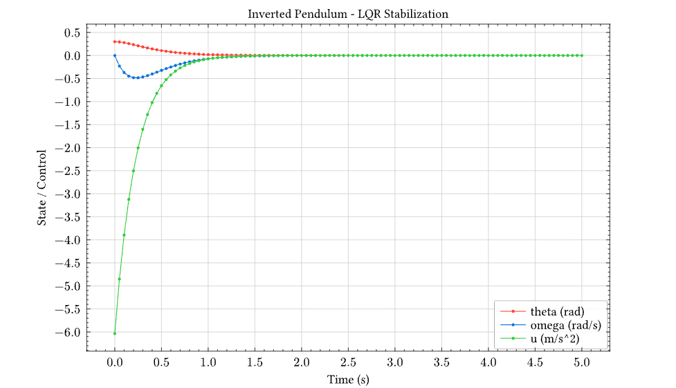
The plot shows:
- θ (red): Angle smoothly decays from 0.3 rad to 0
- ω (blue): Angular velocity with brief negative swing, then settles
- u (green): Initial -6 m/s² control effort (cart accelerates backward to catch falling pendulum), then decays to zero
The LQR controller stabilizes the pendulum in approximately 2 seconds with no overshoot — optimal behavior for the given Q and R weights.
Digital Control: Discrete-Time LQR with Zero-Order Hold
Real controllers are typically implemented digitally with a fixed sample rate. This example shows the same inverted pendulum controlled with a discrete-time LQR designed using the Discrete Algebraic Riccati Equation (DARE).
Key Differences from Continuous Control
| Aspect | Continuous | Discrete |
|---|---|---|
| Design method | lqr() → CARE | dlqr() → DARE |
| System matrices | A, B | Aₐ = eᴬᵀˢ, Bₐ ≈ Ts·B |
| Control update | Continuous | Every Ts seconds (ZOH) |
| Stability check | Re(λ) < 0 | |λ| < 1 |
Complete Example
// Physical parameters
define ell = 0.5 // pendulum length (m)
define grav = 9.81 // gravity (m/s²)
define ts = 0.05 // sample time (s) - 20 Hz
// Continuous-time linearized system
define a_cont = [[0, 1], [grav / ell, 0]]
define b_cont = [[0], [1 / ell]]
// Discretize using matrix exponential
define a_disc = expm(scalar_matrix_mul(ts, a_cont))
define b_disc = scalar_matrix_mul(ts, b_cont)
// LQR weights
define q_matrix = [[1, 0], [0, 0.1]]
define r_matrix = [[1]]
example "Digital LQR with Zero-Order Hold" {
// Compute discrete LQR gains using DARE
let result = dlqr(a_disc, b_disc, q_matrix, r_matrix) in
let k_matrix = nth(result, 0) in
out("Discrete LQR gains K:")
out(k_matrix) // ≈ [[20.18, 4.59]]
// Check closed-loop stability (eigenvalues inside unit circle)
let bk = matmul(b_disc, k_matrix) in
let a_cl = matrix_sub(a_disc, bk) in
out("Closed-loop eigenvalues (|λ| < 1 for stability):")
out(eigenvalues(a_cl))
// Extract gains for simulation
let k1 = nth(nth(k_matrix, 0), 0) in
let k2 = nth(nth(k_matrix, 0), 1) in
// Discrete-time simulation with Euler integration
let n_steps = 100 in
let x0 = [0.1, 0] in // 5.7° initial tilt
// Recursive simulation: each step applies ZOH control
let simulate = lambda acc i .
let prev = nth(acc, length(acc) - 1) in
let t_prev = nth(prev, 0) in
let x_prev = nth(prev, 1) in
let th = nth(x_prev, 0) in
let om = nth(x_prev, 1) in
let u = negate(k1*th + k2*om) in // ZOH control
let th_ddot = (grav/ell)*sin(th) + (u/ell)*cos(th) in
let th_new = th + om*ts in
let om_new = om + th_ddot*ts in
list_append(acc, [[t_prev + ts, [th_new, om_new], u]])
in
let init_u = negate(k1*nth(x0, 0) + k2*nth(x0, 1)) in
let traj = list_fold(simulate, [[0, x0, init_u]], range(0, n_steps)) in
// Extract time series
let times = list_map(lambda p . nth(p, 0), traj) in
let thetas = list_map(lambda p . nth(nth(p, 1), 0), traj) in
let omegas = list_map(lambda p . nth(nth(p, 1), 1), traj) in
let controls = list_map(lambda p . nth(p, 2), traj) in
// Plot with bar chart showing ZOH control action
diagram(
plot(times, thetas, color = "red", label = "theta (rad)"),
plot(times, omegas, color = "blue", label = "omega (rad/s)"),
bar(times, controls, color = "green", label = "u ZOH (m/s^2)",
opacity = 0.3, width = 0.05),
title = "Digital Control - Zero Order Hold (20 Hz)",
xlabel = "Time (s)",
ylabel = "State / Control",
legend = "right + bottom",
width = 16,
height = 10
)
}
Result
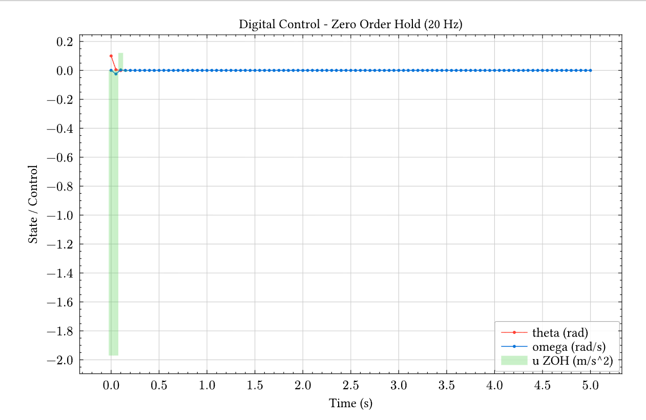
The bar chart shows the zero-order hold (ZOH) nature of digital control — the control signal is constant between sample times (every 50ms). Compare to the smooth continuous control in the previous example.
Note on LQR Tuning
For the inverted pendulum, the gains are relatively insensitive to Q/R weights. This is expected for unstable systems: the Riccati equation solution is dominated by stabilization requirements, leaving little room for performance tuning. For systems where Q/R significantly affects the response, consider stable plants like temperature control or mass-spring-damper systems.
Technical Notes
Adaptive Step Size
The Dormand-Prince 5(4) method adapts its internal step size for accuracy while outputting at the requested dt intervals. This handles stiff transients automatically.
Lambda Closures
The dynamics lambda can capture variables from the enclosing scope:
let k = 2.0 in
let dyn = lambda t y . [negate(k * nth(y, 0))] in
ode45(dyn, [1], [0, 1], 0.1)
// k is captured in the closure
See Also
- LAPACK Functions - Matrix decompositions,
lqr(),dlqr(),eigenvalues() - Jupyter Notebook - Interactive plotting
- Built-in Functions -
list_map,nth,list_fold, etc.
Appendix: Standard Library Reference
The Kleis standard library provides 30 files covering mathematics, physics, and computer science.
File Organization
stdlib/
├── types.kleis // Core type definitions (Bool, Option, List, etc.)
├── prelude.kleis // Core structures and operations
├── minimal_prelude.kleis // Arithmetic, Equatable, Ordered structures
├── func_core.kleis // Higher-order functions (map, fold, etc.)
│
├── # Mathematics
├── complex.kleis // Complex number axioms (ℂ field)
├── rational.kleis // Rational number axioms (ℚ ordered field)
├── matrices.kleis // Matrix algebra (605 lines!)
├── lists.kleis // List operations and axioms
├── sets.kleis // Z3-backed set theory
├── combinatorics.kleis // Permutations, factorials, binomials
├── bigops.kleis // Σ, Π, ∫, lim as polymorphic HOFs
├── bitvector.kleis // Z3 BitVec theory
├── text.kleis // String operations
├── math_functions.kleis // Trig, hyperbolic, special functions
│
├── # Calculus & Analysis
├── calculus.kleis // Derivative/integral axioms, limits
├── calculus_hof.kleis // Derivative as (F → F) → F → F
├── symbolic_diff.kleis // Expression AST with diff(e, x) (differentiation only)
│
├── # Tensors & Differential Geometry
├── tensors.kleis // Abstract tensor algebra
├── tensors_functional.kleis // Pure Kleis tensor operations
├── tensors_concrete.kleis // Component-based tensors for Z3
├── tensors_minimal.kleis // Physics palette notation
├── differential_forms.kleis // Cartan calculus (d, ∧, ⋆, ι)
├── cartan_geometry.kleis // Axiomatic framework for curvature
├── cartan_compute.kleis // Tetrad → Connection → Curvature pipeline
│
├── # Physics
├── maxwell.kleis // Covariant electromagnetism
├── fluid_dynamics.kleis // Navier-Stokes, Bernoulli, Stokes
├── solid_mechanics.kleis // Stress/strain, Von Mises, Mohr-Coulomb
├── quantum.kleis // Hilbert space, Dirac notation, Pauli
├── quantum_minimal.kleis // Physics palette quantum notation
└── cosmology.kleis // Minkowski, de Sitter, FLRW, Schwarzschild
Core Files
types.kleis — Self-Hosted Type System
The type system is defined in Kleis itself:
data Type =
Scalar
| Vector(n: Nat, T)
| Matrix(m: Nat, n: Nat, T)
| Complex
| Set(T: Type)
| List(T: Type)
| Tensor(dims: List(Nat))
data Bool = True | False
data Option(T) = None | Some(value: T)
data Result(T, E) = Ok(value: T) | Err(error: E)
data List(T) = Nil | Cons(head: T, tail: List(T))
prelude.kleis — Core Structures
Defines fundamental mathematical structures:
structure Ring(R) {
zero : R
one : R
operation add : R × R → R
operation mul : R × R → R
operation neg : R → R
axiom add_assoc : ∀(a b c : R). add(add(a, b), c) = add(a, add(b, c))
axiom distributive : ∀(a b c : R). mul(a, add(b, c)) = add(mul(a, b), mul(a, c))
}
func_core.kleis — Functional Primitives
Higher-order functions and function composition:
define compose(f, g) = λ x . f(g(x))
define id(x) = x
define const(x) = λ _ . x
define flip(f) = λ x y . f(y, x)
Mathematics Files
matrices.kleis — Full Matrix Algebra (605 lines)
Comprehensive matrix operations with axioms:
structure Matrix(m: Nat, n: Nat, T) {
operation transpose : Matrix(m, n, T) → Matrix(n, m, T)
operation matmul : Matrix(m, n, T) × Matrix(n, p, T) → Matrix(m, p, T)
operation det : Matrix(n, n, T) → T
operation inv : Matrix(n, n, T) → Matrix(n, n, T)
operation eigenvalues : Matrix(n, n, T) → List(ℂ)
axiom transpose_involution : ∀ A : Matrix(m, n, T) .
transpose(transpose(A)) = A
}
symbolic_diff.kleis — Symbolic Differentiation
Expression AST with pattern-matching differentiation:
data Expression =
ENumber(value : ℝ)
| EVariable(name : String)
| EOperation(name : String, args : List(Expression))
define diff(e, x) = match e {
ENumber(_) => num(0)
| EVariable(name) => if str_eq(name, x) then num(1) else num(0)
| EOperation("plus", [a, b]) => e_add(diff(a, x), diff(b, x))
| EOperation("times", [a, b]) =>
e_add(e_mul(diff(a, x), b), e_mul(a, diff(b, x))) // Product rule
| EOperation("sin", [f]) => e_mul(e_cos(f), diff(f, x)) // Chain rule
// ... more rules
}
calculus_hof.kleis — Derivative as Higher-Order Function
structure Derivative(F) {
operation D : (F → F) → F → F
axiom chain_rule : ∀(f g : F → F)(x : F).
D(compose(f, g))(x) = times(D(f)(g(x)), D(g)(x))
axiom product_rule : ∀(f g : F → F)(x : F).
D(times_fn(f, g))(x) = plus(times(D(f)(x), g(x)), times(f(x), D(g)(x)))
axiom linearity : ∀(f g : F → F)(x : F).
D(plus_fn(f, g))(x) = plus(D(f)(x), D(g)(x))
}
bigops.kleis — Polymorphic Big Operators
Σ, Π, ∫, lim that work on any type with the right structure:
// Summation requires additive monoid (has +, 0)
operation sum_bounds : (ℤ → T) × ℤ × ℤ → T
// Product requires multiplicative monoid (has ×, 1)
operation prod_bounds : (ℤ → T) × ℤ × ℤ → T
// Integral requires Banach space (complete normed vector space)
operation int_bounds : (T → S) × T × T × T → S
// Probability expectation
operation E : (Ω → ℝ) → ℝ
Physics Files
differential_forms.kleis — Cartan Calculus
Full exterior calculus with wedge products, exterior derivative, and Hodge star:
structure WedgeProduct(p: Nat, q: Nat, dim: Nat) {
operation wedge : DifferentialForm(p, dim) → DifferentialForm(q, dim)
→ DifferentialForm(p + q, dim)
axiom graded_antisymmetric : ∀ α β .
wedge(α, β) = scale(power(-1, p*q), wedge(β, α))
}
structure ExteriorDerivative(p: Nat, dim: Nat) {
operation d : DifferentialForm(p, dim) → DifferentialForm(p + 1, dim)
axiom d_squared_zero : ∀ α . d(d(α)) = 0 // Fundamental!
}
// Cartan's Magic Formula: ℒ_X = d ∘ ι_X + ι_X ∘ d
define cartan_magic_impl(X, alpha) =
plus(d(interior(X, alpha)), interior(X, d(alpha)))
cartan_compute.kleis — Schwarzschild Curvature
Complete pipeline from tetrad to Riemann curvature:
define schwarzschild_tetrad(M) =
let f = e_sub(num(1), e_div(e_mul(num(2), M), var("r"))) in
let sqrt_f = e_sqrt(f) in
[
scale1(sqrt_f, dt),
scale1(e_div(num(1), sqrt_f), dr),
scale1(var("r"), dtheta),
scale1(e_mul(var("r"), e_sin(var("theta"))), dphi)
]
define compute_riemann(tetrad) =
let omega = solve_connection(tetrad) in
compute_curvature(omega)
define schwarzschild_curvature(M) = compute_riemann(schwarzschild_tetrad(M))
quantum.kleis — Hilbert Space Formalism
Full quantum mechanics with Dirac notation:
structure Ket(dim: Nat, T) {
operation normalize : Ket(dim, T) → Ket(dim, T)
operation scale : T → Ket(dim, T) → Ket(dim, T)
}
structure Operator(dim: Nat, T) {
operation apply : Operator(dim, T) → Ket(dim, T) → Ket(dim, T)
operation adjoint : Operator(dim, T) → Operator(dim, T)
operation compose : Operator(dim, T) → Operator(dim, T) → Operator(dim, T)
}
structure Commutator(dim: Nat, T) {
operation commutator : Operator(dim, T) → Operator(dim, T) → Operator(dim, T)
// [x̂, p̂] = iℏ (Heisenberg uncertainty!)
}
maxwell.kleis — Covariant Electromagnetism
structure MaxwellInhomogeneous {
operation F : Nat → Nat → ℝ // Field tensor
operation J : Nat → ℝ // 4-current
// ∂_μ F^μν = μ₀ J^ν
axiom maxwell_inhomogeneous : ∀ nu : Nat .
divF(nu) = times(mu0, J(nu))
}
fluid_dynamics.kleis — Navier-Stokes
structure MomentumEquation {
// ρ ∂u_i/∂t + ∂(ρu_i u_j)/∂x_j = -∂p/∂x_i + ∂τ_ij/∂x_j + ρf_i
axiom momentum : ∀ i : Nat .
plus(times(rho, du_dt(i)), div_momentum(i)) =
plus(plus(negate(grad_p(i)), div_tau(i)), times(rho, f(i)))
}
Loading the Standard Library
In files:
import "stdlib/prelude.kleis"
import "stdlib/matrices.kleis"
import "stdlib/symbolic_diff.kleis"
In the REPL:
kleis> :load stdlib/prelude.kleis
Loaded standard library.
See Also
- Cartan Geometry Appendix — Full Schwarzschild example
- ODE Solver Appendix — Control systems with LQR
- LAPACK Functions — Numerical linear algebra
- Built-in Functions — Complete function reference
Appendix: LISP Interpreter in Kleis
This appendix presents a LISP interpreter written entirely in Kleis. This is a demonstration of Kleis’s power as a meta-language — proving that Kleis can parse and execute programs written in other languages.
Note: This is a proof-of-concept, not a production LISP implementation. See Known Limitations for details.
The interpreter includes:
- Recursive descent S-expression parser
- Full evaluator with special forms, arithmetic, comparisons, and list operations
- Lexical closures with
lambda - Recursive functions with
letrec
Running in the REPL
$ cargo run --bin repl
🧮 Kleis REPL v0.1.0
λ> :load examples/meta-programming/lisp_parser.kleis
✅ Loaded: 2 files, 60 functions, 15 structures, 5 data types
λ> :eval run("(+ 2 3)")
✅ VNum(5)
λ> :eval run("(* 4 5)")
✅ VNum(20)
λ> :eval run("(if (< 3 5) 100 200)")
✅ VNum(100)
λ> :eval run("((lambda (x) (* x x)) 7)")
✅ VNum(49)
λ> :eval run("(let ((x 10)) (+ x 5))")
✅ VNum(15)
Factorial
λ> :eval run("(letrec ((fact (lambda (n) (if (<= n 1) 1 (* n (fact (- n 1))))))) (fact 5))")
✅ VNum(120)
Fibonacci
λ> :eval run("(letrec ((fib (lambda (n) (if (< n 2) n (+ (fib (- n 1)) (fib (- n 2))))))) (fib 10))")
✅ VNum(55)
Complete Source Code
The complete LISP interpreter is in examples/meta-programming/lisp_parser.kleis. Below is the full implementation.
Part 1: S-Expression Data Types
import "stdlib/prelude.kleis"
// S-Expression: atoms and lists
data SExpr =
SAtom(value: String)
| SList(elements: List(SExpr))
// Parser result: success with remaining input, or error
data ParseResult =
ParseOK(expr: SExpr, rest: String)
| ParseErr(message: String)
Part 2: Parser Helper Functions
// Check if character is whitespace
define is_ws(c: String) : Bool =
or(eq(c, " "), or(eq(c, "\n"), eq(c, "\t")))
// Check if character is a delimiter
define is_delim(c: String) : Bool =
or(is_ws(c), or(eq(c, "("), eq(c, ")")))
// Skip leading whitespace
define skip_ws(s: String) : String =
if le(strlen(s), 0) then s
else if is_ws(charAt(s, 0)) then skip_ws(substr(s, 1, strlen(s) - 1))
else s
// Read atom characters until delimiter
define read_atom(s: String, acc: String) : ParseResult =
if le(strlen(s), 0) then ParseOK(SAtom(acc), "")
else if is_delim(charAt(s, 0)) then ParseOK(SAtom(acc), s)
else read_atom(substr(s, 1, strlen(s) - 1), concat(acc, charAt(s, 0)))
Part 3: Recursive Descent Parser
// Parse a single S-expression
define parse_sexpr(s: String) : ParseResult =
let trimmed = skip_ws(s) in
if le(strlen(trimmed), 0) then ParseErr("Unexpected end of input")
else if eq(charAt(trimmed, 0), "(") then
parse_list(substr(trimmed, 1, strlen(trimmed) - 1), Nil)
else read_atom(trimmed, "")
// Parse list elements until ")"
define parse_list(s: String, acc: List(SExpr)) : ParseResult =
let trimmed = skip_ws(s) in
if le(strlen(trimmed), 0) then ParseErr("Expected ')'")
else if eq(charAt(trimmed, 0), ")") then
ParseOK(SList(rev(acc)), substr(trimmed, 1, strlen(trimmed) - 1))
else
match parse_sexpr(trimmed) {
ParseOK(expr, rest) => parse_list(rest, Cons(expr, acc))
| ParseErr(msg) => ParseErr(msg)
}
// Reverse a list
define rev(xs: List(SExpr)) : List(SExpr) =
rev_acc(xs, Nil)
define rev_acc(xs: List(SExpr), acc: List(SExpr)) : List(SExpr) =
match xs {
Nil => acc
| Cons(h, t) => rev_acc(t, Cons(h, acc))
}
// User-facing parse function
define parse(s: String) : SExpr =
match parse_sexpr(s) {
ParseOK(expr, rest) => expr
| ParseErr(msg) => SAtom(concat("Error: ", msg))
}
Part 4: LISP Value Types and Environment
// Values in our LISP
data LispVal =
VNum(n: ℤ) // Integer
| VSym(s: String) // Symbol (for errors/unbound)
| VList(xs: List(LispVal)) // List value
| VBool(b: Bool) // Boolean
| VLambda(params: List(String), body: SExpr, env: Env) // Closure
// Environment: list of (name, value) bindings
data Binding = Bind(name: String, val: LispVal)
data Env = Env(bindings: List(Binding))
// Empty environment
define empty_env : Env = Env(Nil)
// Look up a variable in the environment
define lookup(name: String, env: Env) : LispVal =
match env {
Env(bindings) => lookup_list(name, bindings)
}
define lookup_list(name: String, bs: List(Binding)) : LispVal =
match bs {
Nil => VSym(concat("Unbound: ", name))
| Cons(Bind(n, v), rest) =>
if eq(n, name) then v else lookup_list(name, rest)
}
// Extend environment with a new binding
define extend(name: String, val: LispVal, env: Env) : Env =
match env {
Env(bindings) => Env(Cons(Bind(name, val), bindings))
}
// Extend with multiple bindings (for function application)
define extend_all(names: List(String), vals: List(LispVal), env: Env) : Env =
match names {
Nil => env
| Cons(n, ns) =>
match vals {
Nil => env
| Cons(v, vs) => extend_all(ns, vs, extend(n, v, env))
}
}
Part 5: Integer Parsing
define is_digit_char(c: String) : Bool =
or(eq(c, "0"), or(eq(c, "1"), or(eq(c, "2"), or(eq(c, "3"), or(eq(c, "4"),
or(eq(c, "5"), or(eq(c, "6"), or(eq(c, "7"), or(eq(c, "8"), eq(c, "9"))))))))))
define is_number_str(s: String) : Bool =
if le(strlen(s), 0) then false
else if eq(charAt(s, 0), "-") then
if le(strlen(s), 1) then false
else all_digits(substr(s, 1, strlen(s) - 1))
else all_digits(s)
define all_digits(s: String) : Bool =
if le(strlen(s), 0) then true
else if is_digit_char(charAt(s, 0)) then all_digits(substr(s, 1, strlen(s) - 1))
else false
define parse_int(s: String) : ℤ =
if eq(charAt(s, 0), "-") then 0 - parse_int_pos(substr(s, 1, strlen(s) - 1))
else parse_int_pos(s)
define parse_int_pos(s: String) : ℤ =
parse_int_acc(s, 0)
define parse_int_acc(s: String, acc: ℤ) : ℤ =
if le(strlen(s), 0) then acc
else
let d = digit_val(charAt(s, 0)) in
parse_int_acc(substr(s, 1, strlen(s) - 1), acc * 10 + d)
define digit_val(c: String) : ℤ =
if eq(c, "0") then 0 else if eq(c, "1") then 1 else if eq(c, "2") then 2
else if eq(c, "3") then 3 else if eq(c, "4") then 4 else if eq(c, "5") then 5
else if eq(c, "6") then 6 else if eq(c, "7") then 7 else if eq(c, "8") then 8
else 9
Part 6: Main Evaluator
define eval_lisp(expr: SExpr, env: Env) : LispVal =
match expr {
SAtom(s) =>
if is_number_str(s) then VNum(parse_int(s))
else if eq(s, "true") then VBool(true)
else if eq(s, "false") then VBool(false)
else lookup(s, env)
| SList(elements) => eval_list(elements, env)
}
define eval_list(elements: List(SExpr), env: Env) : LispVal =
match elements {
Nil => VList(Nil) // Empty list is a value
| Cons(head, rest) => eval_form(head, rest, env)
}
// Evaluate a special form or function call
define eval_form(head: SExpr, args: List(SExpr), env: Env) : LispVal =
match head {
SAtom(op) =>
// Special forms
if eq(op, "if") then eval_if(args, env)
else if eq(op, "quote") then eval_quote(args)
else if eq(op, "lambda") then eval_lambda(args, env)
else if eq(op, "let") then eval_let(args, env)
else if eq(op, "letrec") then eval_letrec(args, env)
// Arithmetic
else if eq(op, "+") then eval_add(args, env)
else if eq(op, "-") then eval_sub(args, env)
else if eq(op, "*") then eval_mul(args, env)
else if eq(op, "/") then eval_div(args, env)
// Comparison
else if eq(op, "<") then eval_lt(args, env)
else if eq(op, ">") then eval_gt(args, env)
else if eq(op, "=") then eval_eq(args, env)
else if eq(op, "<=") then eval_le(args, env)
else if eq(op, ">=") then eval_ge(args, env)
// List operations
else if eq(op, "list") then eval_list_op(args, env)
else if eq(op, "car") then eval_car(args, env)
else if eq(op, "cdr") then eval_cdr(args, env)
else if eq(op, "cons") then eval_cons(args, env)
else if eq(op, "null?") then eval_null(args, env)
// Function call
else eval_call(op, args, env)
| SList(_) =>
// First element is an expression (e.g., lambda)
let fn_val = eval_lisp(head, env) in
eval_apply(fn_val, args, env)
}
Part 7: Special Forms
define eval_if(args: List(SExpr), env: Env) : LispVal =
match args {
Cons(cond, Cons(then_br, Cons(else_br, Nil))) =>
let cv = eval_lisp(cond, env) in
if is_truthy(cv) then eval_lisp(then_br, env) else eval_lisp(else_br, env)
| _ => VSym("Error: if requires 3 arguments")
}
define is_truthy(v: LispVal) : Bool =
match v {
VBool(b) => b
| VNum(n) => not(eq(n, 0))
| VList(Nil) => false
| VList(_) => true
| VSym(_) => false
| VLambda(_, _, _) => true
}
define eval_quote(args: List(SExpr)) : LispVal =
match args {
Cons(expr, Nil) => sexpr_to_val(expr)
| _ => VSym("Error: quote requires 1 argument")
}
define sexpr_to_val(expr: SExpr) : LispVal =
match expr {
SAtom(s) => if is_number_str(s) then VNum(parse_int(s)) else VSym(s)
| SList(elements) => VList(map_sexpr_to_val(elements))
}
define map_sexpr_to_val(xs: List(SExpr)) : List(LispVal) =
match xs {
Nil => Nil
| Cons(h, t) => Cons(sexpr_to_val(h), map_sexpr_to_val(t))
}
define eval_lambda(args: List(SExpr), env: Env) : LispVal =
match args {
Cons(SList(params), Cons(body, Nil)) =>
VLambda(extract_param_names(params), body, env)
| _ => VSym("Error: lambda requires (params) body")
}
define extract_param_names(params: List(SExpr)) : List(String) =
match params {
Nil => Nil
| Cons(SAtom(name), rest) => Cons(name, extract_param_names(rest))
| _ => Nil
}
define eval_let(args: List(SExpr), env: Env) : LispVal =
match args {
Cons(SList(bindings), Cons(body, Nil)) =>
let new_env = eval_let_bindings(bindings, env) in
eval_lisp(body, new_env)
| _ => VSym("Error: let requires ((bindings)) body")
}
define eval_let_bindings(bindings: List(SExpr), env: Env) : Env =
match bindings {
Nil => env
| Cons(SList(Cons(SAtom(name), Cons(val_expr, Nil))), rest) =>
let val = eval_lisp(val_expr, env) in
eval_let_bindings(rest, extend(name, val, env))
| _ => env
}
// letrec: evaluate lambda in an environment that already contains the binding
// This enables recursion: (letrec ((fact (lambda (n) ...))) (fact 5))
define eval_letrec(args: List(SExpr), env: Env) : LispVal =
match args {
Cons(SList(bindings), Cons(body, Nil)) =>
let rec_env = eval_letrec_bindings(bindings, env) in
eval_lisp(body, rec_env)
| _ => VSym("Error: letrec requires ((bindings)) body")
}
define eval_letrec_bindings(bindings: List(SExpr), env: Env) : Env =
match bindings {
Nil => env
| Cons(SList(Cons(SAtom(name), Cons(SList(Cons(SAtom(lambda_kw),
Cons(SList(params), Cons(body, Nil)))), Nil))), rest) =>
let dummy_env = extend(name, VSym("placeholder"), env) in
let lambda_val = VLambda(extract_param_names(params), body, dummy_env) in
let new_env = extend(name, lambda_val, env) in
let fixed_lambda = VLambda(extract_param_names(params), body, new_env) in
eval_letrec_bindings(rest, extend(name, fixed_lambda, env))
| _ => env
}
Part 8: Arithmetic Operations
define eval_add(args: List(SExpr), env: Env) : LispVal =
match args {
Cons(a, Cons(b, Nil)) =>
match eval_lisp(a, env) {
VNum(x) => match eval_lisp(b, env) {
VNum(y) => VNum(x + y)
| _ => VSym("Error: + requires numbers")
}
| _ => VSym("Error: + requires numbers")
}
| _ => VSym("Error: + requires 2 arguments")
}
define eval_sub(args: List(SExpr), env: Env) : LispVal =
match args {
Cons(a, Cons(b, Nil)) =>
match eval_lisp(a, env) {
VNum(x) => match eval_lisp(b, env) {
VNum(y) => VNum(x - y)
| _ => VSym("Error: - requires numbers")
}
| _ => VSym("Error: - requires numbers")
}
| _ => VSym("Error: - requires 2 arguments")
}
define eval_mul(args: List(SExpr), env: Env) : LispVal =
match args {
Cons(a, Cons(b, Nil)) =>
match eval_lisp(a, env) {
VNum(x) => match eval_lisp(b, env) {
VNum(y) => VNum(x * y)
| _ => VSym("Error: * requires numbers")
}
| _ => VSym("Error: * requires numbers")
}
| _ => VSym("Error: * requires 2 arguments")
}
define eval_div(args: List(SExpr), env: Env) : LispVal =
match args {
Cons(a, Cons(b, Nil)) =>
match eval_lisp(a, env) {
VNum(x) => match eval_lisp(b, env) {
VNum(y) => if eq(y, 0) then VSym("Error: division by zero")
else VNum(x / y)
| _ => VSym("Error: / requires numbers")
}
| _ => VSym("Error: / requires numbers")
}
| _ => VSym("Error: / requires 2 arguments")
}
Part 9: Comparison Operations
define eval_lt(args: List(SExpr), env: Env) : LispVal =
match args {
Cons(a, Cons(b, Nil)) =>
match eval_lisp(a, env) {
VNum(x) => match eval_lisp(b, env) {
VNum(y) => VBool(lt(x, y))
| _ => VSym("Error: < requires numbers")
}
| _ => VSym("Error: < requires numbers")
}
| _ => VSym("Error: < requires 2 arguments")
}
define eval_gt(args: List(SExpr), env: Env) : LispVal =
match args {
Cons(a, Cons(b, Nil)) =>
match eval_lisp(a, env) {
VNum(x) => match eval_lisp(b, env) {
VNum(y) => VBool(gt(x, y))
| _ => VSym("Error: > requires numbers")
}
| _ => VSym("Error: > requires numbers")
}
| _ => VSym("Error: > requires 2 arguments")
}
define eval_eq(args: List(SExpr), env: Env) : LispVal =
match args {
Cons(a, Cons(b, Nil)) =>
match eval_lisp(a, env) {
VNum(x) => match eval_lisp(b, env) {
VNum(y) => VBool(eq(x, y))
| _ => VSym("Error: = requires numbers")
}
| _ => VSym("Error: = requires numbers")
}
| _ => VSym("Error: = requires 2 arguments")
}
define eval_le(args: List(SExpr), env: Env) : LispVal =
match args {
Cons(a, Cons(b, Nil)) =>
match eval_lisp(a, env) {
VNum(x) => match eval_lisp(b, env) {
VNum(y) => VBool(le(x, y))
| _ => VSym("Error: <= requires numbers")
}
| _ => VSym("Error: <= requires numbers")
}
| _ => VSym("Error: <= requires 2 arguments")
}
define eval_ge(args: List(SExpr), env: Env) : LispVal =
match args {
Cons(a, Cons(b, Nil)) =>
match eval_lisp(a, env) {
VNum(x) => match eval_lisp(b, env) {
VNum(y) => VBool(ge(x, y))
| _ => VSym("Error: >= requires numbers")
}
| _ => VSym("Error: >= requires numbers")
}
| _ => VSym("Error: >= requires 2 arguments")
}
Part 10: List Operations
define eval_list_op(args: List(SExpr), env: Env) : LispVal =
VList(eval_all(args, env))
define eval_all(args: List(SExpr), env: Env) : List(LispVal) =
match args {
Nil => Nil
| Cons(h, t) => Cons(eval_lisp(h, env), eval_all(t, env))
}
define eval_car(args: List(SExpr), env: Env) : LispVal =
match args {
Cons(lst, Nil) =>
match eval_lisp(lst, env) {
VList(Cons(h, _)) => h
| _ => VSym("Error: car requires non-empty list")
}
| _ => VSym("Error: car requires 1 argument")
}
define eval_cdr(args: List(SExpr), env: Env) : LispVal =
match args {
Cons(lst, Nil) =>
match eval_lisp(lst, env) {
VList(Cons(_, t)) => VList(t)
| _ => VSym("Error: cdr requires non-empty list")
}
| _ => VSym("Error: cdr requires 1 argument")
}
define eval_cons(args: List(SExpr), env: Env) : LispVal =
match args {
Cons(h, Cons(t, Nil)) =>
let hv = eval_lisp(h, env) in
match eval_lisp(t, env) {
VList(lst) => VList(Cons(hv, lst))
| _ => VSym("Error: cons requires list as second arg")
}
| _ => VSym("Error: cons requires 2 arguments")
}
define eval_null(args: List(SExpr), env: Env) : LispVal =
match args {
Cons(lst, Nil) =>
match eval_lisp(lst, env) {
VList(Nil) => VBool(true)
| VList(_) => VBool(false)
| _ => VSym("Error: null? requires list")
}
| _ => VSym("Error: null? requires 1 argument")
}
Part 11: Function Application
define eval_call(name: String, args: List(SExpr), env: Env) : LispVal =
let fn_val = lookup(name, env) in
eval_apply(fn_val, args, env)
define eval_apply(fn_val: LispVal, args: List(SExpr), env: Env) : LispVal =
match fn_val {
VLambda(params, body, closure_env) =>
let arg_vals = eval_all(args, env) in
// Merge current env into closure env for recursive calls
let merged_env = merge_envs(env, closure_env) in
let new_env = extend_all(params, arg_vals, merged_env) in
eval_lisp(body, new_env)
| VSym(msg) => VSym(msg) // Error propagation
| _ => VSym("Error: not a function")
}
// Merge two environments: first takes precedence
// This allows letrec functions to see their own definitions
define merge_envs(e1: Env, e2: Env) : Env =
match e1 {
Env(b1) => match e2 {
Env(b2) => Env(append_bindings(b1, b2))
}
}
define append_bindings(b1: List(Binding), b2: List(Binding)) : List(Binding) =
match b1 {
Nil => b2
| Cons(h, t) => Cons(h, append_bindings(t, b2))
}
Part 12: User-Facing Run Function
// Run a LISP program from string
define run(code: String) : LispVal =
eval_lisp(parse(code), empty_env)
// Run with an environment (for multiple expressions)
define run_with_env(code: String, env: Env) : LispVal =
eval_lisp(parse(code), env)
Known Limitations
This LISP interpreter is a demonstration, not a production-level implementation. It proves that Kleis can parse and execute programs, but has known limitations:
| Issue | Description | Status |
|---|---|---|
| Trailing junk ignored | parse("(+ 1 2) garbage") parses successfully, ignoring “garbage” | Known |
| Errors as atoms | Parse errors return SAtom("Error: ...") instead of a proper error type | Known |
| No quote syntax | Standard LISP '(1 2 3) is not supported; use (list 1 2 3) instead | Known |
| Limited special forms | Only if, lambda, let, letrec, define are implemented | By design |
| No macros | LISP macros are not supported | By design |
| Integer-only arithmetic | No floating-point numbers | By design |
Why These Limitations Exist
This interpreter demonstrates Kleis’s meta-language capabilities, not LISP completeness. The goal is to show:
- Kleis can parse arbitrary grammars using recursive descent
- Kleis can build and traverse ASTs (S-expressions as Kleis data types)
- Kleis can execute recursive programs via
:eval - Kleis is Turing-complete
For production LISP, use Racket, SBCL, or Clojure.
Summary
This LISP interpreter demonstrates that Kleis is Turing-complete and can serve as a host language for other programming languages. The implementation uses:
| Feature | Kleis Construct |
|---|---|
| Data types | data SExpr, data LispVal, data Env |
| Pattern matching | match expr { ... } |
| Recursion | Recursive function definitions |
| Higher-order functions | lambda, closures with captured environments |
| String operations | charAt, substr, concat, strlen |
| List operations | Cons, Nil, pattern matching on lists |
Key Insights
-
:evalenables execution — The:evalREPL command executes Kleis functions directly, without going through Z3’s symbolic unrolling. -
Environment merging for recursion —
letrecworks by merging the current environment (which contains the function binding) into the closure’s environment. -
60 pure functions — The entire interpreter is implemented in ~560 lines of pure functional Kleis code.
-
Meta-circular potential — With minor extensions, this could interpret a subset of Kleis itself, demonstrating meta-circularity.
VS Code Debugging
This appendix explains how to set up and use the VS Code debugger with Kleis.
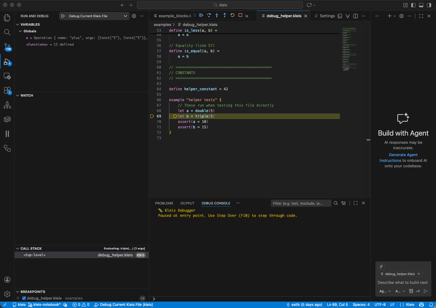
VS Code debugging a Kleis file: breakpoint on line 69, Variables panel showing expression AST, Call Stack showing evaluation context, and Debug Console with status messages.
Prerequisites
- VS Code installed
- Kleis extension installed (provides syntax highlighting + debugging)
- Kleis binaries built:
cargo build --release --bin kleis --bin kleis-lsp
Extension Setup
The Kleis VS Code extension is located in vscode-kleis/. Install it:
cd vscode-kleis
npm install
npm run compile
code --install-extension kleis-*.vsix
Or for development, open the extension folder in VS Code and press F5 to launch an Extension Development Host.
Workspace Settings
Create .vscode/settings.json in your project to configure the extension:
{
"kleis.serverPath": "${workspaceFolder}/target/release/kleis",
"kleis.replPath": "${workspaceFolder}/target/release/repl",
"kleis.trace.server": "off"
}
Settings Reference
| Setting | Description |
|---|---|
kleis.serverPath | Path to the kleis binary (used for LSP and DAP) |
kleis.replPath | Path to the repl binary (used for REPL panel) |
kleis.trace.server | Logging level: "off", "messages", or "verbose" |
Note: Use absolute paths for reliability. Example for a typical setup:
{
"kleis.serverPath": "/Users/yourname/git/kleis/target/release/kleis",
"kleis.replPath": "/Users/yourname/git/kleis/target/release/repl",
"kleis.trace.server": "off"
}
Set "kleis.trace.server": "verbose" when debugging extension issues.
Launch Configuration
Create .vscode/launch.json in your project:
{
"version": "0.2.0",
"configurations": [
{
"type": "kleis",
"request": "launch",
"name": "Debug Kleis File",
"program": "${file}",
"stopOnEntry": false
}
]
}
Configuration Options
| Option | Type | Description |
|---|---|---|
program | string | Path to .kleis file to debug |
stopOnEntry | boolean | Stop at first line (default: false) |
Setting Breakpoints
Click in the gutter (left margin) next to any line in an example block:
example "my test" {
let x = 5 // ← Click here to set breakpoint
let y = double(x) // ← Or here
assert(y = 10)
}
Where Breakpoints Work
| Location | Works? | Notes |
|---|---|---|
| Inside example blocks | ✅ Yes | let, assert, expressions |
| Function body lines | ✅ Yes | Stops when function is called |
| Top-level definitions | ❌ No | Declarations, not executable |
| Imported files | ✅ Yes | Set breakpoints in helper files |
Breakpoints in Imported Files
You can set breakpoints in imported files:
// helpers.kleis
define double(n) =
n + n // ← Breakpoint here catches all calls to double()
// main.kleis
import "helpers.kleis"
example "cross-file breakpoint" {
let x = double(5) // Stops at the breakpoint in helpers.kleis
}
Tip: Open the imported file and set breakpoints before starting the debug session.
Starting a Debug Session
- Open a
.kleisfile with example blocks - Set breakpoints on lines you want to inspect
- Press F5 or click Run → Start Debugging
- Select “Debug Kleis File” configuration
Debug Controls
| Key | Action | Description |
|---|---|---|
| F5 | Continue | Run until next breakpoint |
| F10 | Step Over | Execute current line, don’t enter functions |
| F11 | Step Into | Enter function calls |
| Shift+F11 | Step Out | Finish current function, return to caller |
| Shift+F5 | Stop | End debug session |
Inspecting Variables
The Variables panel (left sidebar) shows:
- Local variables — Let bindings in current scope
- Function parameters — Arguments passed to current function
- Inferred types — When available, types are displayed
Important: Variables are displayed as AST expressions, not just values:
example "inspection demo" {
let x = 5
let y = x + 1
// Variables panel shows:
// x = Const("5")
// y = Operation { name: "plus", args: [Const("5"), Const("1")] }
}
Type-Aware Variable Display
When type information is available, variables show their inferred types:
example "typed variables" {
let M = matrix2x3([[1,2,3],[4,5,6]])
let v = vector3([1, 2, 3])
let c = complex(1, 2)
// Variables panel shows:
// M : Matrix(2,3,ℝ) = [[1,2,3],[4,5,6]]
// v : Vector(3,ℝ) = [1, 2, 3]
// c : ℂ = 1+2i
}
This is intentional! Kleis is a symbolic mathematics system. Variables hold expressions that represent mathematical objects, not just computed values. This enables:
- Symbolic manipulation — See the structure of expressions
- Z3 verification — Pass expressions to the theorem prover
- Provenance tracking — Understand where values came from
- Type checking — Verify types match expectations
Call Stack
The Call Stack panel shows the execution path:
fibonacci (n=5) ← Currently here
fibonacci (n=6)
example "fib test" ← Entry point
Click any frame to see its local variables and source location.
Cross-File Debugging
When stepping into imported functions, VS Code opens the source file:
// main.kleis
import "helpers.kleis"
example "cross-file" {
let result = helper_function(5) // ← Step Into (F11)
// VS Code opens helpers.kleis at helper_function definition
}
How It Works
Every expression carries its source location (line, column, file path). When the evaluator processes an expression from an imported file, the debugger reports that file’s location to VS Code, which opens it automatically.
Debug Console
The Debug Console (bottom panel) shows:
- Evaluation progress
- Assertion results (pass/fail)
- Error messages
You can also evaluate expressions in the console during a paused debug session.
Assert with Z3 Verification
New in v0.93: Assertions in example blocks use Z3 for symbolic verification!
How It Works
When you write assert(expr):
- Concrete values — Checked via structural equality
- Symbolic expressions — Verified using Z3 theorem prover
structure CommutativeRing(R) {
operation (+) : R × R → R
axiom commutativity: ∀(a b : R). a + b = b + a
}
example "symbolic verification" {
// ✅ Z3 verifies using commutativity axiom!
assert(x + y = y + x)
// ❌ Z3 disproves with counterexample
// assert(x + y = y + y) // "Counterexample: y!1 -> 1, x!0 -> 0"
// ✅ Concrete: structural equality
let a = 5
assert(a = 5)
}
Assertion Results
| Result | Badge | Meaning |
|---|---|---|
Passed | ✓ | Concrete values match structurally |
Verified | ✓ | Z3 proved the symbolic claim |
Failed { expected, actual } | ✗ | Concrete values differ |
Disproved { counterexample } | ✗ | Z3 found a counterexample |
Unknown | ✗ | Could not verify (treated as failure) |
Note: The debugger displays verification badges (✓/✗) next to assertion variables in the Variables panel, so you can see at a glance which assertions passed or failed.
Requirements
- Structure axioms must be defined for the operations used
- Z3 must be able to load the relevant axioms
- Works best with algebraic properties (commutativity, associativity, etc.)
Numerical Computations
For concrete numerical computations, build with the numerical feature:
cargo build --release --features numerical
This enables LAPACK-backed operations:
example "numerical" {
let A = Matrix(2, 2, [4, 1, 1, 4])
// Compute eigenvalues (requires numerical feature)
let eigs = eigenvalues(A)
// eigs = [5, 3]
// Matrix multiplication
let B = Matrix(2, 2, [1, 0, 0, 2])
let C = matmul(A, B)
// SVD decomposition
let usv = svd(A) // Returns [U, S, V]
}
Available Numerical Operations
| Operation | Description |
|---|---|
eigenvalues(M) | Compute eigenvalues |
eig(M) | Eigenvalues and eigenvectors |
svd(M) | Singular value decomposition |
solve(A, b) | Solve linear system Ax = b |
inv(M) | Matrix inverse |
det(M) | Determinant |
cholesky(M) | Cholesky decomposition |
qr(M) | QR factorization |
matmul(A, B) | Matrix multiplication |
Note: Numerical operations require concrete values. Symbolic matrices remain symbolic.
Troubleshooting
Breakpoints Not Hitting
Problem: Breakpoint shows as gray (unverified) or never hits.
Solutions:
- Ensure breakpoint is on a line inside an example block
- Ensure the example block is actually executed
- Rebuild the Kleis binaries:
cargo build --release
“File not found” Errors
Problem: Debugger can’t find imported files.
Solutions:
- Use relative paths in imports:
import "stdlib/complex.kleis" - Run debug session from the project root directory
- Check that the imported file exists at the specified path
Slow Stepping
Problem: Each step takes several seconds.
Solutions:
- Use release builds:
cargo build --release - Avoid stepping through deeply recursive functions
- Use “Step Over” (F10) instead of “Step Into” (F11) for library functions
Debug Session Won’t Start
Problem: F5 does nothing or shows an error.
Solutions:
- Check
.vscode/launch.jsonexists and is valid JSON - Ensure Kleis extension is installed and enabled
- Check the Output panel (View → Output → Kleis) for error messages
- Verify binaries exist:
ls target/release/kleis*
Architecture
The debugging system uses the Debug Adapter Protocol (DAP):
┌─────────────┐ DAP ┌──────────────┐
│ VS Code │ ←───────────────→ │ kleis server │
│ (client) │ JSON-RPC │ (adapter) │
└─────────────┘ └──────────────┘
│
▼
┌──────────────┐
│ Evaluator │
│ + DebugHook │
└──────────────┘
- VS Code sends DAP commands (setBreakpoints, next, stepIn, etc.)
- Kleis server translates to evaluator debug hook calls
- Evaluator pauses at breakpoints, reports current expression’s span
- Server sends stopped events with location (line, column, file)
- VS Code highlights the current line
Source Span Tracking
The key to accurate debugging is SourceSpan:
#![allow(unused)]
fn main() {
pub struct SourceSpan {
pub line: u32,
pub column: u32,
pub end_line: u32,
pub end_column: u32,
pub file: Option<Arc<PathBuf>>, // File path (Arc for cheap cloning)
}
}Every Expression node has an optional span. The parser attaches the span during parsing. When evaluating, the span travels with the expression, so the debugger always knows the source location.
Understanding Symbolic Debugging
Kleis debugging differs from traditional debuggers because Kleis is a symbolic mathematics system, not an imperative programming language.
What “Execution” Means in Kleis
In Kleis, “execution” means symbolic evaluation:
- Substitution — Replace function calls with their definitions
- Pattern matching — Dispatch based on structure
- Simplification — Apply algebraic rules
There’s no “program counter” moving through instructions. Instead, expressions transform into simpler expressions.
Variables Hold Expressions, Not Values
let y = sin(x) + cos(x)
// y doesn't hold a number
// y holds: Operation { name: "plus", args: [sin(x), cos(x)] }
This is intentional! It enables:
- Passing expressions to Z3 for verification
- Symbolic differentiation, integration
- Algebraic manipulation
When to Use the Debugger
| Use Case | Debugger Helps? |
|---|---|
| Understanding expression evaluation | ✅ Excellent |
| Verifying axiom applications | ✅ See Z3 results |
| Finding structural issues | ✅ See AST in Variables |
| Computing numeric values | 🔶 Need numerical feature |
| Traditional imperative debugging | ❌ Wrong mental model |
Tips for Effective Debugging
- Start with simple examples — Debug small example blocks first
- Use Step Over for library code — Don’t step into stdlib functions unless needed
- Watch the Variables panel — See how expressions transform as you step
- Set multiple breakpoints — Mark key points in your logic
- Use the Call Stack — Understand the substitution chain
- Think symbolically — Variables hold AST, not computed values
- Use Z3 for verification — Let
assert()prove symbolic claims
See Also
- Example Blocks — How to write debuggable code
- The REPL — Interactive exploration
- Grammar Reference — Full language syntax
Appendix: Cartan Geometry and Tensor Computation
This appendix demonstrates Kleis’s capability to perform symbolic tensor calculus for general relativity, computing actual curvature tensors from metric specifications.
Overview
Kleis implements Cartan’s formalism for differential geometry:
Metric → Tetrad → Connection → Curvature → Ricci → Einstein
This is the same computational pipeline used in research-grade general relativity software like xAct (Mathematica) and Cadabra.
The Cartan Pipeline
1. Expression AST
Symbolic expressions are represented using the Expression algebraic data type, consistent with kleis_in_kleis.kleis:
data Expression =
ENumber(value : ℝ)
| EVariable(name : String)
| EOperation(name : String, args : List(Expression))
This representation allows any operation to be encoded uniformly via EOperation. Helper constructors provide cleaner syntax:
// Value constructors
define num(n) = ENumber(n)
define var(x) = EVariable(x)
// Operation constructors (e_ prefix avoids builtin conflicts)
define e_add(a, b) = EOperation("plus", Cons(a, Cons(b, Nil)))
define e_mul(a, b) = EOperation("times", Cons(a, Cons(b, Nil)))
define e_pow(a, b) = EOperation("power", Cons(a, Cons(b, Nil)))
define e_sin(a) = EOperation("sin", Cons(a, Nil))
define e_cos(a) = EOperation("cos", Cons(a, Nil))
define e_sqrt(a) = EOperation("sqrt", Cons(a, Nil))
// ... etc
2. Symbolic Differentiation
The diff function computes derivatives by pattern matching on the Expression AST:
define diff(e, var_name) = match e {
// Constant rule: d/dx(c) = 0
ENumber(_) => num(0)
// Variable rule: d/dx(x) = 1, d/dx(y) = 0 if y ≠ x
// Note: str_eq() is used for concrete string comparison
EVariable(name) => if str_eq(name, var_name) then num(1) else num(0)
// Operation rules - dispatch by operation name
EOperation(op_name, args) => diff_op(op_name, args, var_name)
}
define diff_op(op_name, args, var_name) = match op_name {
"plus" => match args {
Cons(f, Cons(g, Nil)) => e_add(diff(f, var_name), diff(g, var_name))
| _ => num(0)
}
"times" => match args {
// Product rule: d/dx(f * g) = f' * g + f * g'
Cons(f, Cons(g, Nil)) =>
e_add(e_mul(diff(f, var_name), g), e_mul(f, diff(g, var_name)))
| _ => num(0)
}
"power" => match args {
// Power rule with constant exponent
Cons(f, Cons(ENumber(n), Nil)) =>
e_mul(e_mul(num(n), e_pow(f, num(n - 1))), diff(f, var_name))
// General power rule
| _ => num(0)
}
"sin" => match args {
Cons(f, Nil) => e_mul(e_cos(f), diff(f, var_name))
| _ => num(0)
}
// ... more rules
}
Note: We use
str_eq(name, var_name)instead of pattern matching because Kleis patterns bind variables rather than compare them. Thestr_eqbuiltin provides concrete string equality.
3. Differential Forms
1-forms and 2-forms are represented as coefficient lists:
// 1-form: ω = ω_t dt + ω_r dr + ω_θ dθ + ω_φ dφ
// Represented as [ω_t, ω_r, ω_θ, ω_φ]
define dt = [num(1), num(0), num(0), num(0)]
define dr = [num(0), num(1), num(0), num(0)]
define dtheta = [num(0), num(0), num(1), num(0)]
define dphi = [num(0), num(0), num(0), num(1)]
4. Exterior Derivative
// d(f) = ∂f/∂t dt + ∂f/∂r dr + ∂f/∂θ dθ + ∂f/∂φ dφ
define d0(f) = [
simplify(diff_t(f)),
simplify(diff_r(f)),
simplify(diff_theta(f)),
simplify(diff_phi(f))
]
// Coordinate-specific derivatives
define diff_t(e) = diff(e, "t")
define diff_r(e) = diff(e, "r")
define diff_theta(e) = diff(e, "theta")
define diff_phi(e) = diff(e, "phi")
5. Wedge Product
// (α ∧ β)_μν = α_μ β_ν - α_ν β_μ
define wedge(a, b) =
let a0 = nth(a, 0) in let a1 = nth(a, 1) in
let a2 = nth(a, 2) in let a3 = nth(a, 3) in
let b0 = nth(b, 0) in let b1 = nth(b, 1) in
let b2 = nth(b, 2) in let b3 = nth(b, 3) in
[
[num(0),
simplify(e_sub(e_mul(a0, b1), e_mul(a1, b0))),
...],
...
]
Example: Schwarzschild Black Hole
The Schwarzschild metric describes spacetime around a non-rotating black hole:
ds² = -(1 - 2M/r)dt² + dr²/(1 - 2M/r) + r²dθ² + r²sin²θ dφ²
Tetrad Definition
define schwarzschild_tetrad(M) =
let f = e_sub(num(1), e_div(e_mul(num(2), M), var("r"))) in
let sqrt_f = e_sqrt(f) in
[
scale1(sqrt_f, dt), // e⁰ = √f dt
scale1(e_div(num(1), sqrt_f), dr), // e¹ = dr/√f
scale1(var("r"), dtheta), // e² = r dθ
scale1(e_mul(var("r"), e_sin(var("theta"))), dphi) // e³ = r sin(θ) dφ
]
Computing Curvature
define compute_riemann(tetrad) =
let omega = solve_connection(tetrad) in
compute_curvature(omega)
define schwarzschild_curvature(M) =
compute_riemann(schwarzschild_tetrad(M))
Results
| Computation | Size | Time |
|---|---|---|
| Tetrad | ~300 chars | instant |
| Connection ω^a_b | ~2,400 chars | ~1s |
| Curvature R^a_b | ~22,000 chars | ~4s |
Literature Verification
The computed results match known properties from the literature:
Minkowski (Flat Space)
- Expected: All curvature components = 0
- Computed: 238/256 components are
ENumber(0)✓ - Reference: Misner, Thorne, Wheeler “Gravitation” (1973)
Schwarzschild
- Expected: Curvature depends on M, r, angular coordinates
- Computed: Contains
EVariable("M"),EVariable("r"),sin,cos✓ - Expected: Contains metric factor √(1-2M/r)
- Computed: Contains
e_sqrt(e_sub(num(1), e_div(...)))✓ - Reference: Carroll “Spacetime and Geometry” (2004)
Implementation Notes
Why e_* Prefix?
Functions like pow, add, mul conflict with Kleis builtins. When you write pow(var("x"), num(2)), Kleis interprets pow as the built-in power operation and tries to compute EVariable("x") ^ ENumber(2) numerically—which fails.
The e_* prefix (e_pow, e_add, etc.) ensures these are treated as user-defined functions that construct EOperation nodes.
Why str_eq Instead of Pattern Matching?
In Kleis (and ML-family languages), pattern variables bind rather than compare:
// This BINDS 'x' to whatever name contains, always matches!
EVariable(name) => match name { x => num(1) | _ => num(0) }
// This COMPARES name to var_name using str_eq
EVariable(name) => if str_eq(name, var_name) then num(1) else num(0)
The str_eq builtin provides concrete string equality that returns true or false.
Z3 Verification
While the Cartan computation runs in the Kleis evaluator, the results can be verified using Z3:
// Verify Riemann tensor symmetries
axiom riemann_antisym : ∀ R μ ν ρ σ .
component(R, μ, ν, ρ, σ) = negate(component(R, ν, μ, ρ, σ))
// Verify Bianchi identity
axiom bianchi : ∀ R λ ρ σ μ ν .
plus(plus(
nabla(R, λ, ρ, σ, μ, ν),
nabla(R, ρ, σ, λ, μ, ν)),
nabla(R, σ, λ, ρ, μ, ν)) = 0
Files
| File | Description |
|---|---|
stdlib/symbolic_diff.kleis | Expression AST and symbolic differentiation |
stdlib/cartan_geometry.kleis | Axiomatic framework (structures, axioms for Z3) |
stdlib/cartan_compute.kleis | Computational implementation (actually computes) |
tests/symbolic_diff_test.rs | 25 tests for differentiation |
tests/cartan_compute_test.rs | 22 tests including literature verification |
Two Complementary Approaches
cartan_geometry.kleis defines the theory:
structure CurvatureForm(dim: Nat) {
operation curvature : List(List(DifferentialForm(1, dim))) → ...
axiom curvature_def : ∀ omega . R^a_b = dω^a_b + ω^a_c ∧ ω^c_b
axiom bianchi : ... // Formal Bianchi identity for Z3
}
cartan_compute.kleis provides the computation:
define compute_curvature(omega) = [
[curvature_ab(omega, 0, 0), curvature_ab(omega, 0, 1), ...],
... // Actually evaluates to Expression values
]
Both now use the same Expression AST from symbolic_diff.kleis.
Research Applications
| Domain | Application |
|---|---|
| General Relativity | Compute curvature for new metrics |
| Cosmology | Verify FLRW, de Sitter models |
| Modified Gravity | Check f(R) theory consistency |
| Numerical Relativity | Verify constraint equations |
| Education | Interactive GR computations |
Comparison to Other Tools
| Tool | Symbolic | Verification | Notes |
|---|---|---|---|
| Mathematica + xAct | ✓✓✓ | ✗ | Industry standard, expensive |
| Cadabra | ✓✓ | ✗ | Open source tensor algebra |
| SageMath | ✓✓ | ✗ | General purpose |
| Kleis | ✓✓ | ✓✓ | Combines both! |
Kleis occupies a unique niche: symbolic mathematics with formal verification.