Appendix: ODE Solver
Kleis provides numerical integration of ordinary differential equations through the ode45 function. This implements the Dormand-Prince 5(4) adaptive step-size method, suitable for non-stiff initial value problems.
Note: The ODE solver is available when Kleis is compiled with the
numericalfeature.
Basic Usage
ode45(dynamics, y0, t_span, dt)
| Argument | Type | Description |
|---|---|---|
dynamics | Lambda | System dynamics function (see below) |
y0 | List | Initial state vector |
t_span | [t0, t1] | Time interval |
dt | Number | Output time step (optional, default 0.1) |
The Dynamics Function
The dynamics argument is a lambda of the form:
lambda t y . [dy0/dt, dy1/dt, ...]
where:
tis the current time (scalar)yis the current state vector[y0, y1, ...]- The return value is a list of derivatives, same length as
y
For higher-order ODEs, convert to a system of first-order equations by introducing auxiliary state variables:
| Original Equation | State Vector | Dynamics Return |
|---|---|---|
| y’ = f(t, y) | [y] | [f(t, y)] |
| y’’ = f(t, y, y’) | [y, y'] | [y', f(t, y, y')] |
| y’‘’ = f(t, y, y’, y’’) | [y, y', y''] | [y', y'', f(...)] |
Example: The second-order equation y’’ + y = 0 becomes:
- State:
[y, v]where v = y’ - Dynamics:
[v, -y]since y’ = v and v’ = -y
Accessing State Components
Use nth(list, index) to extract elements from the state vector (0-indexed):
lambda t y .
  let x = nth(y, 0) in    // first component
  let v = nth(y, 1) in    // second component
  [v, negate(x)]          // return [dx/dt, dv/dt]
Returns
A list of [t, [y0, y1, ...]] pairs representing the trajectory.
Simple Example: Exponential Decay
The equation dy/dt = -y with y(0) = 1 has the solution y(t) = e^(-t).
let decay = lambda t y . [negate(nth(y, 0))] in
let traj = ode45(decay, [1.0], [0, 3], 0.5) in
traj
// → [[0, [1.0]], [0.5, [0.606...]], [1.0, [0.367...]], ...]
Harmonic Oscillator
A second-order ODE like x’’ = -x is converted to a first-order system:
- State:
[x, v]where v = x’ - Dynamics:
[x', v'] = [v, -x]
let oscillator = lambda t y .
  let x = nth(y, 0) in
  let v = nth(y, 1) in
  [v, negate(x)]
in
ode45(oscillator, [1, 0], [0, 6.28], 0.1)
// Completes one period, returns to [1, 0]
Control Systems: Inverted Pendulum with LQR
This example demonstrates a complete control system workflow:
- System modeling - Nonlinear pendulum dynamics
- LQR design - Optimal feedback gains via CARE
- Simulation - Closed-loop response with
ode45 - Visualization - State and control trajectories
Problem Setup
An inverted pendulum on an acceleration-controlled cart:
- State:
[θ, ω]where θ is angle from vertical, ω is angular velocity - Control: u = cart acceleration (m/s²)
- Dynamics: θ’’ = (g/L)·sin(θ) + (u/L)·cos(θ)
Linearized System
Around the upright equilibrium (θ = 0):
A = [0,    1  ]     B = [0  ]
    [g/L,  0  ]         [1/L]
With L = 0.5m and g = 9.81 m/s², the open-loop eigenvalues are ±4.43 — one unstable pole.
Complete Example
// Physical parameters
define ell = 0.5        // pendulum length (m)
define grav = 9.81      // gravity (m/s²)

// Linearized system matrices
define a_matrix = [[0, 1], [grav / ell, 0]]
define b_matrix = [[0], [1 / ell]]

// LQR cost weights
define q_matrix = [[10, 0], [0, 1]]  // Penalize angle more than velocity
define r_matrix = [[1]]

// Helper functions
define get_time(pt) = nth(pt, 0)
define get_theta(pt) = nth(nth(pt, 1), 0)
define get_omega(pt) = nth(nth(pt, 1), 1)

example "LQR pendulum stabilization" {
  // Compute optimal LQR gains by solving CARE
  let result = lqr(a_matrix, b_matrix, q_matrix, r_matrix) in
  let k1 = nth(nth(nth(result, 0), 0), 0) in
  let k2 = nth(nth(nth(result, 0), 0), 1) in

  out("LQR gains: k1, k2 =")
  out(k1)  // ≈ 20.12
  out(k2)  // ≈ 4.60

  out("Open-loop eigenvalues (unstable):")
  out(eigenvalues(a_matrix))  // [4.43, -4.43]

  // Nonlinear dynamics with LQR feedback: u = -K·x
  let dyn = lambda t y .
    let th = nth(y, 0) in
    let om = nth(y, 1) in
    let u = negate(k1*th + k2*om) in
    [om, (grav/ell)*sin(th) + (u/ell)*cos(th)]
  in

  // Simulate from 17° initial tilt
  let traj = ode45(dyn, [0.3, 0], [0, 5], 0.05) in

  // Extract time series
  let times = list_map(lambda p . get_time(p), traj) in
  let thetas = list_map(lambda p . get_theta(p), traj) in
  let omegas = list_map(lambda p . get_omega(p), traj) in
  let controls = list_map(lambda p .
    negate(20.12*get_theta(p) + 4.60*get_omega(p)), traj) in

  // Plot state and control
  diagram(
    plot(times, thetas, color = "red", label = "theta (rad)"),
    plot(times, omegas, color = "blue", label = "omega (rad/s)"),
    plot(times, controls, color = "green", label = "u (m/s^2)"),
    title = "Inverted Pendulum - LQR Stabilization",
    xlabel = "Time (s)",
    ylabel = "State / Control",
    legend = "right + bottom",
    width = 16,
    height = 10
  )
}
Result
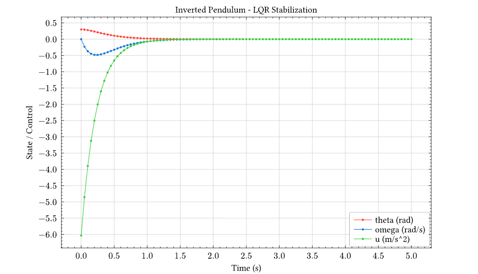
The plot shows:
- θ (red): Angle smoothly decays from 0.3 rad to 0
- ω (blue): Angular velocity with brief negative swing, then settles
- u (green): Initial -6 m/s² control effort (cart accelerates backward to catch falling pendulum), then decays to zero
The LQR controller stabilizes the pendulum in approximately 2 seconds with no overshoot — optimal behavior for the given Q and R weights.
Digital Control: Discrete-Time LQR with Zero-Order Hold
Real controllers are typically implemented digitally with a fixed sample rate. This example shows the same inverted pendulum controlled with a discrete-time LQR designed using the Discrete Algebraic Riccati Equation (DARE).
Key Differences from Continuous Control
| Aspect | Continuous | Discrete |
|---|---|---|
| Design method | lqr() → CARE | dlqr() → DARE |
| System matrices | A, B | Aₐ = eᴬᵀˢ, Bₐ ≈ Ts·B |
| Control update | Continuous | Every Ts seconds (ZOH) |
| Stability check | Re(λ) < 0 | |λ| < 1 |
Complete Example
// Physical parameters
define ell = 0.5        // pendulum length (m)
define grav = 9.81      // gravity (m/s²)
define ts = 0.05        // sample time (s) - 20 Hz

// Continuous-time linearized system
define a_cont = [[0, 1], [grav / ell, 0]]
define b_cont = [[0], [1 / ell]]

// Discretize using matrix exponential
define a_disc = expm(scalar_matrix_mul(ts, a_cont))
define b_disc = scalar_matrix_mul(ts, b_cont)

// LQR weights
define q_matrix = [[1, 0], [0, 0.1]]
define r_matrix = [[1]]

example "Digital LQR with Zero-Order Hold" {
  // Compute discrete LQR gains using DARE
  let result = dlqr(a_disc, b_disc, q_matrix, r_matrix) in
  let k_matrix = nth(result, 0) in

  out("Discrete LQR gains K:")
  out(k_matrix)  // ≈ [[20.18, 4.59]]

  // Check closed-loop stability (eigenvalues inside unit circle)
  let bk = matmul(b_disc, k_matrix) in
  let a_cl = matrix_sub(a_disc, bk) in
  out("Closed-loop eigenvalues (|λ| < 1 for stability):")
  out(eigenvalues(a_cl))

  // Extract gains for simulation
  let k1 = nth(nth(k_matrix, 0), 0) in
  let k2 = nth(nth(k_matrix, 0), 1) in

  // Discrete-time simulation with Euler integration
  let n_steps = 100 in
  let x0 = [0.1, 0] in  // 5.7° initial tilt

  // Recursive simulation: each step applies ZOH control
  let simulate = lambda acc i .
    let prev = nth(acc, length(acc) - 1) in
    let t_prev = nth(prev, 0) in
    let x_prev = nth(prev, 1) in
    let th = nth(x_prev, 0) in
    let om = nth(x_prev, 1) in
    let u = negate(k1*th + k2*om) in  // ZOH control
    let th_ddot = (grav/ell)*sin(th) + (u/ell)*cos(th) in
    let th_new = th + om*ts in
    let om_new = om + th_ddot*ts in
    list_append(acc, [[t_prev + ts, [th_new, om_new], u]])
  in

  let init_u = negate(k1*nth(x0, 0) + k2*nth(x0, 1)) in
  let traj = list_fold(simulate, [[0, x0, init_u]], range(0, n_steps)) in

  // Extract time series
  let times = list_map(lambda p . nth(p, 0), traj) in
  let thetas = list_map(lambda p . nth(nth(p, 1), 0), traj) in
  let omegas = list_map(lambda p . nth(nth(p, 1), 1), traj) in
  let controls = list_map(lambda p . nth(p, 2), traj) in

  // Plot with bar chart showing ZOH control action
  diagram(
    plot(times, thetas, color = "red", label = "theta (rad)"),
    plot(times, omegas, color = "blue", label = "omega (rad/s)"),
    bar(times, controls, color = "green", label = "u ZOH (m/s^2)",
        opacity = 0.3, width = 0.05),
    title = "Digital Control - Zero Order Hold (20 Hz)",
    xlabel = "Time (s)",
    ylabel = "State / Control",
    legend = "right + bottom",
    width = 16,
    height = 10
  )
}
Result
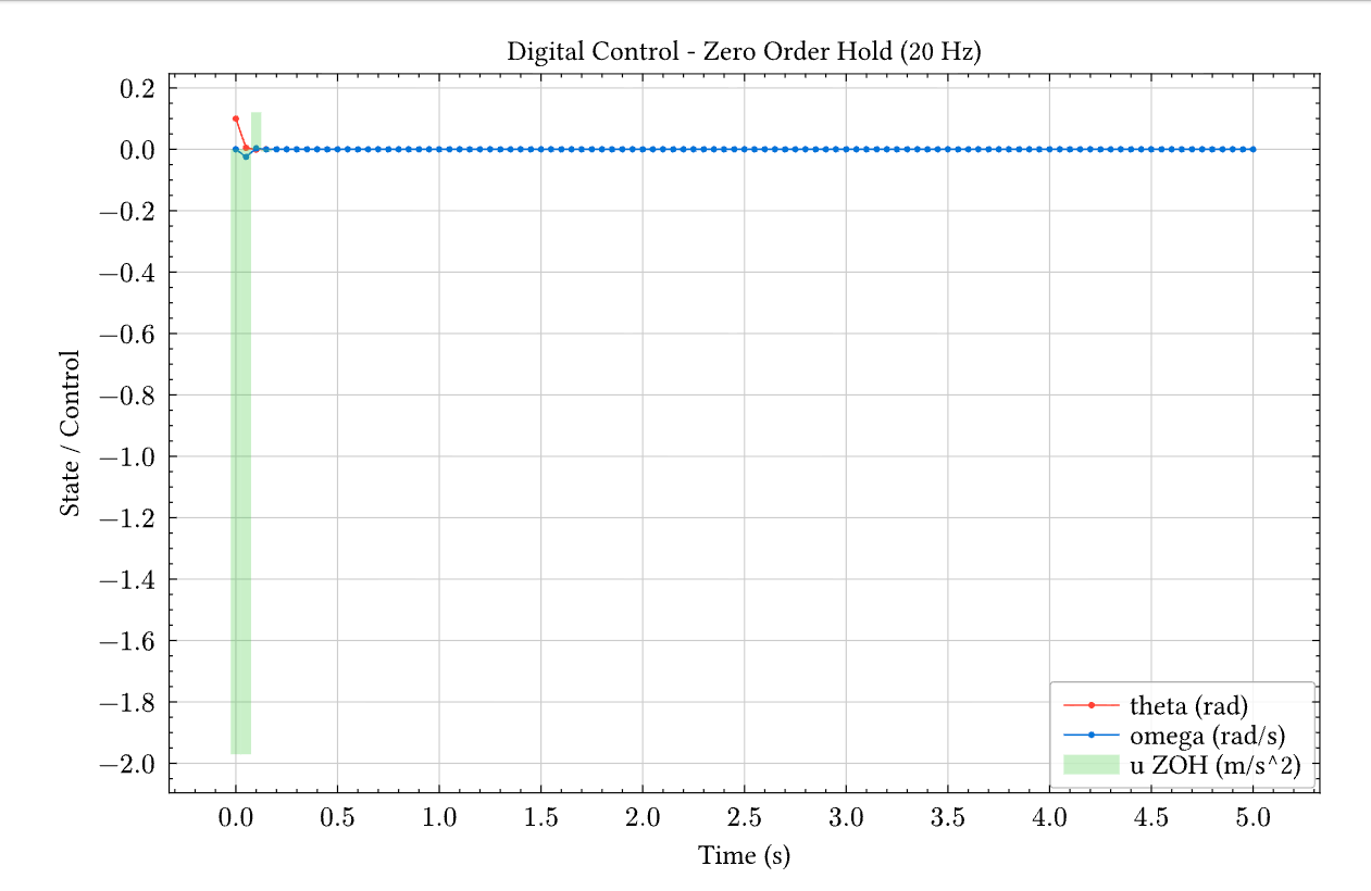
The bar chart shows the zero-order hold (ZOH) nature of digital control — the control signal is constant between sample times (every 50ms). Compare to the smooth continuous control in the previous example.
Note on LQR Tuning
For the inverted pendulum, the gains are relatively insensitive to Q/R weights. This is expected for unstable systems: the Riccati equation solution is dominated by stabilization requirements, leaving little room for performance tuning. For systems where Q/R significantly affects the response, consider stable plants like temperature control or mass-spring-damper systems.
Technical Notes
Adaptive Step Size
The Dormand-Prince 5(4) method adapts its internal step size for accuracy while outputting at the requested dt intervals. This handles stiff transients automatically.
Lambda Closures
The dynamics lambda can capture variables from the enclosing scope:
let k = 2.0 in
let dyn = lambda t y . [negate(k * nth(y, 0))] in
ode45(dyn, [1], [0, 1], 0.1)
// k is captured in the closure
See Also
- LAPACK Functions - Matrix decompositions,
lqr(),dlqr(),eigenvalues() - Jupyter Notebook - Interactive plotting
- Built-in Functions -
list_map,nth,list_fold, etc.